Visualisation
Overview
Sherpa has support for different plot backends, at present limited to matplotlib and ChIPS. Interactive visualizations of images is provided by DS9 - an Astronomical image viewer - if installed, whilst there is limited support for visualizing two-dimensional data sets with matplotlib. The classes described in this document do not need to be used, since the data can be plotted directly, but they do provide some conveniences.
The basic approach to creating a visualization using these classes is:
- create an instance of the relevant class (e.g.
DataPlot);- send it the necessary data with the
prepare()method (optional);- perform any necessary calculation with the
calc()method (optional);- and plot the data with the
plot()orcontour()methods (or theoverplot(), andovercontour()variants).
Note
The sherpa.plot module also includes error-estimation routines, such as the IntervalProjection class. This is mixing analysis with visualization, which may not be ideal.
Example
>>> import numpy as np
>>> edges = np.asarray([-10, -5, 5, 12, 17, 20, 30, 56, 60])
>>> y = np.asarray([28, 62, 17, 4, 2, 4, 55, 125])
>>> from sherpa.data import Data1DInt
>>> d = Data1DInt('example histogram', edges[:-1], edges[1:], y)
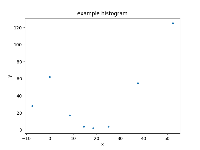
>>> from sherpa.plot import DataPlot
>>> dplot = DataPlot()
>>> dplot.prepare(d)
>>> dplot.plot()

Some text.
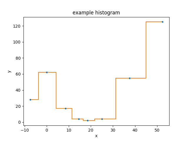
>>> from sherpa.plot import Histogram
>>> hplot = Histogram()
>>> hplot.overplot(d.xlo, d.xhi, d.y)

Some more text.
>>> from sherpa.models.basic import Const1D, Gauss1D
>>> mdl = Const1D('base') - Gauss1D('line')
>>> for p, v in zip(mdl.pars, [10, 25, 22, 10]):
...     p.val = v
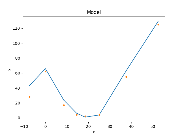
>>> from sherpa.plot import ModelPlot
>>> mplot = ModelPlot()
>>> mplot.prepare(d, mdl)
>>> mplot.plot()
>>> dplot.overplot()

Blah.
>>> from sherpa.optmethods import NelderMead
>>> from sherpa.stats import Cash
>>> from sherpa.fit import Fit
>>> f = Fit(d, mdl, stat=Cash(), method=NelderMead())
>>> f.fit()
>>> from sherpa.plot import IntervalProjection
>>> iproj = IntervalProjection()
>>> iproj.calc(f, mdl.pars[2])
WARNING: hard minimum hit for parameter base.c0
WARNING: hard maximum hit for parameter base.c0
WARNING: hard minimum hit for parameter line.fwhm
WARNING: hard maximum hit for parameter line.fwhm
WARNING: hard minimum hit for parameter line.ampl
WARNING: hard maximum hit for parameter line.ampl
>>> iproj.plot()
Hmmmm. Not good results. Need to reevaluate the data beng used here.
Reference/API
- The sherpa.plot module
- Confidence1D
- IntervalProjection
- IntervalUncertainty
- Confidence2D
- RegionProjection
- RegionUncertainty
- Contour
- DataContour
- PSFContour
- FitContour
- ModelContour
- RatioContour
- ResidContour
- SourceContour
- Histogram
- Plot
- DataPlot
- PSFPlot
- FitPlot
- ModelPlot
- ChisqrPlot
- ComponentModelPlot
- DelchiPlot
- RatioPlot
- ResidPlot
- SourcePlot
- ComponentSourcePlot
- SplitPlot
- JointPlot
- Point
- Class Inheritance Diagram
- The sherpa.astro.plot module