What data is to be fit?¶

The Sherpa Data class is used to carry around the data to be fit: this includes the independent axis (or axes), the dependent axis (the data), and any necessary metadata. Although the design of Sherpa supports multiple-dimensional data sets, the current classes only support one- and two-dimensional data sets.

Overview¶

The following modules are assumed to have been imported:

>>> import numpy as np
>>> import matplotlib.pyplot as plt
>>> from sherpa.stats import LeastSq
>>> from sherpa.optmethods import LevMar
>>> from sherpa import data

Names¶

The first argument to any of the Data classes is the name of the data set. This is used for display purposes only, and can be useful to identify which data set is in use. It is stored in the name attribute of the object, and can be changed at any time.

The independent axis¶

The independent axis - or axes - of a data set define the grid over which the model is to be evaluated. It is referred to as x, x0, x1, ... depending on the dimensionality of the data (for binned datasets there are lo and hi variants).

Although dense multi-dimensional data sets can be stored as arrays with dimensionality greater than one, the internal representation used by Sherpa is often a flattened - i.e. one-dimensional - version.

The dependent axis¶

This refers to the data being fit, and is referred to as y.

Unbinned data¶

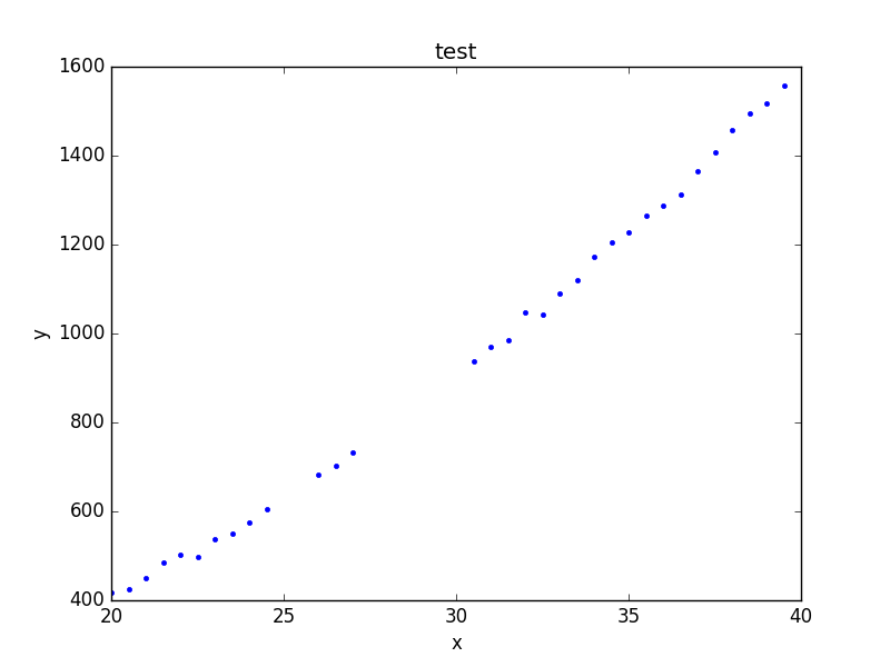
Unbinned data sets - defined by classes which do not end in the name Int - represent point values; that is, the the data value is the value at the coordinates given by the independent axis. Examples of unbinned data classes are Data1D and Data2D.

>>> np.random.seed(0)
>>> x = np.arange(20, 40, 0.5)
>>> y = x**2 + np.random.normal(0, 10, size=x.size)
>>> d1 = data.Data1D('test', x, y)
>>> print(d1)
name      = test
x         = Float64[40]
y         = Float64[40]
staterror = None
syserror  = None

Binned data¶

Binned data sets represent values that are defined over a range, such as a histogram. The integrated model classes end in Int: examples are Data1DInt and Data2DInt.

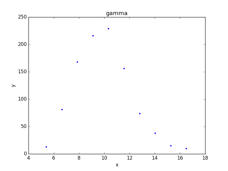
It can be a useful optimisation to treat a binned data set as an unbinned one, since it avoids having to estimate the integral of the model over each bin. It depends in part on how the bin size compares to the scale over which the model changes.

>>> z = np.random.gamma(20, scale=0.5, size=1000)
>>> (y, edges) = np.histogram(z)
>>> d2 = data.Data1DInt('gamma', edges[:-1], edges[1:], y)
>>> print(d2)
name      = gamma
xlo       = Float64[10]
xhi       = Float64[10]
y         = Int64[10]
staterror = None
syserror  = None
>>> plt.bar(d2.xlo, d2.y, d2.xhi - d2.xlo);

Errors¶

There is support for both statistical and systematic errors by either using the staterror and syserror parameters when creating the data object, or by changing the staterror and syserror attributes of the object.

Filtering data¶

Sherpa supports filtering data sets; that is, temporarily removing parts of the data (perhaps because there are problems, or to help restrict parameter values).

The mask attribute indicates whether a filter has been applied: if it returns True then no filter is set, otherwise it is a bool array where False values indicate those elements that are to be ignored. The ignore() and notice() methods are used to define the ranges to exclude or include. For example, the following hides those values where the independent axis values are between 21.2 and 22.8:

>>> d1.ignore(21.2, 22.8)
>>> d1.x[np.invert(d1.mask)]
array([ 21.5,  22. ,  22.5])

After this, a fit to the data will ignore these values, as shown below, where the number of degrees of freedom of the first fit, which uses the filtered data, is three less than the fit to the full data set (the call to notice() removes the filter since no arguments were given):

>>> from sherpa.models import Polynom1D
>>> from sherpa.fit import Fit
>>> mdl = Polynom1D()
>>> mdl.c2.thaw()
>>> fit = Fit(d1, mdl, stat=LeastSq(), method=LevMar())
>>> res1 = fit.fit()

>>> d1.notice()
>>> res2 = fit.fit()

>>> print("Degrees of freedom: {} vs {}".format(res1.dof, res2.dof))
Degrees of freedom: 35 vs 38

Note

It’s a bit confusing since not always clear where a given attribute or method is defined. There’s also get_filter/get_filter_expr to deal with. Also filter/apply_filter.

Visualizing a data set¶

The data objects contain several methods which can be used to visualize the data, but do not provide any direct plotting or display capabilities. There are low-level routines which provide access to the data - these include the to_plot() and to_contour() methods - but the preferred approach is to use the classes defined in the sherpa.plot module, which are described in the visualization section:

>>> from sherpa.plot import DataPlot
>>> pdata = DataPlot()
>>> pdata.prepare(d2)
>>> pdata.plot()

Although the data represented by d2 is a histogram, the values are displayed at the center of the bin.

The plot objects automatically handle any filters applied to the data, as shown below.

>>> d1.ignore(25, 30)
>>> d1.notice(26, 27)
>>> pdata.prepare(d1)
>>> pdata.plot()

Note

The plot object stores the data given in the prepare() call, so that changes to the underlying objects will not be reflected in future calls to plot() unless a new call to prepare() is made.

>>> d1.notice()

At this point, a call to pdata.plot() would re-create the previous plot, even though the filter has been removed from the underlying data object.

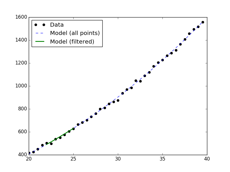
Evaluating a model¶

The eval_model() and eval_model_to_fit() methods can be used to evaluate a model on the grid defined by the data set. The first version uses the full grid, whereas the second respects any filtering applied to the data.

>>> d1.notice(22, 25)
>>> y1 = d1.eval_model(mdl)
>>> y2 = d1.eval_model_to_fit(mdl)
>>> x2 = d1.x[d1.mask]
>>> plt.plot(d1.x, d1.y, 'ko', label='Data')
>>> plt.plot(d1.x, y1, '--', label='Model (all points)')
>>> plt.plot(x2, y2, linewidth=2, label='Model (filtered)')
>>> plt.legend(loc=2)

Reference/API¶

Note

There are a bunch of methods that seem out of place; e.g. Data1D has get_x0 even though it’s not ND!