Reference/API
Capabilities
astropy.modeling Package
This subpackage provides a framework for representing models and performing model evaluation and fitting. It supports 1D and 2D models and fitting with parameter constraints. It has some predefined models and fitting routines.
Functions
custom_model(*args[, fit_deriv]) |
Create a model from a user defined function. |
is_separable(transform) |
A separability test for the outputs of a transform. |
separability_matrix(transform) |
Compute the correlation between outputs and inputs. |
Classes
CompoundModel(op, left, right[, name, inverse]) |
Base class for compound models. |
Fittable1DModel(*args[, meta, name]) |
Base class for one-dimensional fittable models. |
Fittable2DModel(*args[, meta, name]) |
Base class for two-dimensional fittable models. |
FittableModel(*args[, meta, name]) |
Base class for models that can be fitted using the built-in fitting algorithms. |
InputParameterError |
Used for incorrect input parameter values and definitions. |
Model(*args[, meta, name]) |
Base class for all models. |
ModelDefinitionError |
Used for incorrect models definitions. |
Parameter([name, description, default, …]) |
Wraps individual parameters. |
ParameterError |
Generic exception class for all exceptions pertaining to Parameters. |
Class Inheritance Diagram
astropy.modeling.mappings Module
Special models useful for complex compound models where control is needed over which outputs from a source model are mapped to which inputs of a target model.
Classes
Mapping(mapping[, n_inputs, name, meta]) |
Allows inputs to be reordered, duplicated or dropped. |
Identity(n_inputs[, name, meta]) |
Returns inputs unchanged. |
Class Inheritance Diagram
astropy.modeling.fitting Module
This module implements classes (called Fitters) which combine optimization
algorithms (typically from scipy.optimize) with statistic functions to perform
fitting. Fitters are implemented as callable classes. In addition to the data
to fit, the __call__ method takes an instance of
FittableModel as input, and returns a copy of the
model with its parameters determined by the optimizer.
Optimization algorithms, called “optimizers” are implemented in
optimizers and statistic functions are in
statistic. The goal is to provide an easy to extend
framework and allow users to easily create new fitters by combining statistics
with optimizers.
There are two exceptions to the above scheme.
LinearLSQFitter uses Numpy’s lstsq
function. LevMarLSQFitter uses
leastsq which combines optimization and statistic in one
implementation.
Classes
LinearLSQFitter() |
A class performing a linear least square fitting. |
LevMarLSQFitter() |
Levenberg-Marquardt algorithm and least squares statistic. |
FittingWithOutlierRemoval(fitter, outlier_func) |
This class combines an outlier removal technique with a fitting procedure. |
SLSQPLSQFitter() |
SLSQP optimization algorithm and least squares statistic. |
SimplexLSQFitter() |
Simplex algorithm and least squares statistic. |
JointFitter(models, jointparameters, initvals) |
Fit models which share a parameter. |
Fitter(optimizer, statistic) |
Base class for all fitters. |
Class Inheritance Diagram
astropy.modeling.optimizers Module
Optimization algorithms used in fitting.
Classes
Optimization(opt_method) |
Base class for optimizers. |
SLSQP() |
Sequential Least Squares Programming optimization algorithm. |
Simplex() |
Neald-Mead (downhill simplex) algorithm. |
Class Inheritance Diagram
astropy.modeling.statistic Module
Statistic functions used in fitting.
Functions
leastsquare(measured_vals, updated_model, …) |
Least square statistic with optional weights. |
astropy.modeling.tabular Module
Tabular models.
Tabular models of any dimension can be created using tabular_model.
For convenience Tabular1D and Tabular2D are provided.
Examples
>>> table = np.array([[ 3.,  0.,  0.],
...                  [ 0.,  2.,  0.],
...                  [ 0.,  0.,  0.]])
>>> points = ([1, 2, 3], [1, 2, 3])
>>> t2 = Tabular2D(points, lookup_table=table, bounds_error=False,
...                fill_value=None, method='nearest')
Functions
tabular_model(dim[, name]) |
Make a Tabular model where n_inputs is based on the dimension of the lookup_table. |
astropy.modeling.separable Module
Functions to determine if a model is separable, i.e. if the model outputs are independent.
It analyzes n_inputs, n_outputs and the operators
in a compound model by stepping through the transforms
and creating a coord_matrix of shape (n_outputs, n_inputs).
Each modeling operator is represented by a function which
takes two simple models (or two coord_matrix arrays) and
returns an array of shape (n_outputs, n_inputs).
Functions
is_separable(transform) |
A separability test for the outputs of a transform. |
separability_matrix(transform) |
Compute the correlation between outputs and inputs. |
Pre-Defined Models
astropy.modeling.functional_models Module
Mathematical models.
Classes
AiryDisk2D([amplitude, x_0, y_0, radius]) |
Two dimensional Airy disk model. |
Moffat1D([amplitude, x_0, gamma, alpha]) |
One dimensional Moffat model. |
Moffat2D([amplitude, x_0, y_0, gamma, alpha]) |
Two dimensional Moffat model. |
Box1D([amplitude, x_0, width]) |
One dimensional Box model. |
Box2D([amplitude, x_0, y_0, x_width, y_width]) |
Two dimensional Box model. |
Const1D([amplitude]) |
One dimensional Constant model. |
Const2D([amplitude]) |
Two dimensional Constant model. |
Ellipse2D([amplitude, x_0, y_0, a, b, theta]) |
A 2D Ellipse model. |
Disk2D([amplitude, x_0, y_0, R_0]) |
Two dimensional radial symmetric Disk model. |
Gaussian1D([amplitude, mean, stddev]) |
One dimensional Gaussian model. |
Gaussian2D([amplitude, x_mean, y_mean, …]) |
Two dimensional Gaussian model. |
Linear1D([slope, intercept]) |
One dimensional Line model. |
Lorentz1D([amplitude, x_0, fwhm]) |
One dimensional Lorentzian model. |
MexicanHat1D([amplitude, x_0, sigma]) |
One dimensional Mexican Hat model. |
MexicanHat2D([amplitude, x_0, y_0, sigma]) |
Two dimensional symmetric Mexican Hat model. |
RedshiftScaleFactor([z]) |
One dimensional redshift scale factor model. |
Multiply([factor]) |
Multiply a model by a quantity or number. |
Planar2D([slope_x, slope_y, intercept]) |
Two dimensional Plane model. |
Scale([factor]) |
Multiply a model by a dimensionless factor. |
Sersic1D([amplitude, r_eff, n]) |
One dimensional Sersic surface brightness profile. |
Sersic2D([amplitude, r_eff, n, x_0, y_0, …]) |
Two dimensional Sersic surface brightness profile. |
Shift([offset]) |
Shift a coordinate. |
Sine1D([amplitude, frequency, phase]) |
One dimensional Sine model. |
Trapezoid1D([amplitude, x_0, width, slope]) |
One dimensional Trapezoid model. |
TrapezoidDisk2D([amplitude, x_0, y_0, R_0, …]) |
Two dimensional circular Trapezoid model. |
Ring2D([amplitude, x_0, y_0, r_in, width, r_out]) |
Two dimensional radial symmetric Ring model. |
Voigt1D([x_0, amplitude_L, fwhm_L, fwhm_G]) |
One dimensional model for the Voigt profile. |
KingProjectedAnalytic1D([amplitude, r_core, …]) |
Projected (surface density) analytic King Model. |
Class Inheritance Diagram
astropy.modeling.powerlaws Module
Power law model variants
Classes
PowerLaw1D([amplitude, x_0, alpha]) |
One dimensional power law model. |
BrokenPowerLaw1D([amplitude, x_break, …]) |
One dimensional power law model with a break. |
SmoothlyBrokenPowerLaw1D([amplitude, …]) |
One dimensional smoothly broken power law model. |
ExponentialCutoffPowerLaw1D([amplitude, …]) |
One dimensional power law model with an exponential cutoff. |
LogParabola1D([amplitude, x_0, alpha, beta]) |
One dimensional log parabola model (sometimes called curved power law). |
Class Inheritance Diagram
astropy.modeling.blackbody Module
Model and functions related to blackbody radiation.
Blackbody Radiation
Blackbody flux is calculated with Planck law (Rybicki & Lightman 1979):
where the unit of \(B_{\lambda}(T)\) is
\(erg \; s^{-1} cm^{-2} \mathring{A}^{-1} sr^{-1}\), and
\(B_{\nu}(T)\) is \(erg \; s^{-1} cm^{-2} Hz^{-1} sr^{-1}\).
blackbody_lambda() and
blackbody_nu() calculate the
blackbody flux for \(B_{\lambda}(T)\) and \(B_{\nu}(T)\),
respectively.
For blackbody representation as a model, see BlackBody1D.
Examples
>>> import numpy as np
>>> from astropy import units as u
>>> from astropy.modeling.blackbody import blackbody_lambda, blackbody_nu
Calculate blackbody flux for 5000 K at 100 and 10000 Angstrom while suppressing any Numpy warnings:
>>> wavelengths = [100, 10000] * u.AA
>>> temperature = 5000 * u.K
>>> with np.errstate(all='ignore'):
...     flux_lam = blackbody_lambda(wavelengths, temperature)
...     flux_nu = blackbody_nu(wavelengths, temperature)
>>> flux_lam
<Quantity [  1.27452545e-108,  7.10190526e+005] erg / (Angstrom cm2 s sr)>
>>> flux_nu
<Quantity [  4.25135927e-123,  2.36894060e-005] erg / (cm2 Hz s sr)>
Alternatively, the same results for flux_nu can be computed using
BlackBody1D with blackbody representation as a model. The difference between
this and the former approach is in one additional step outlined as follows:
>>> from astropy import constants as const
>>> from astropy.modeling import models
>>> temperature = 5000 * u.K
>>> bolometric_flux = const.sigma_sb * temperature ** 4 / np.pi
>>> bolometric_flux.to(u.erg / (u.cm * u.cm * u.s))
<Quantity 1.12808367e+10 erg / (cm2 s)>
>>> wavelengths = [100, 10000] * u.AA
>>> bb_astro = models.BlackBody1D(temperature, bolometric_flux=bolometric_flux)
>>> bb_astro(wavelengths).to(u.erg / (u.cm * u.cm * u.Hz * u.s)) / u.sr
<Quantity [4.25102471e-123, 2.36893879e-005] erg / (cm2 Hz s sr)>
where bb_astro(wavelengths) computes the equivalent result as flux_nu above.
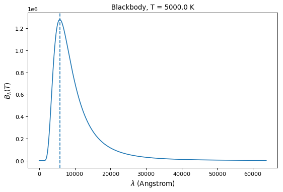
Plot a blackbody spectrum for 5000 K:
Note that an array of temperatures can also be given instead of a single
temperature. In this case, the Numpy broadcasting rules apply: for instance, if
the frequency and temperature have the same shape, the output will have this
shape too, while if the frequency is a 2-d array with shape (n, m) and the
temperature is an array with shape (m,), the output will have a shape
(n, m).
See Also
Rybicki, G. B., & Lightman, A. P. 1979, Radiative Processes in Astrophysics (New York, NY: Wiley)
Functions
blackbody_nu(in_x, temperature) |
Calculate blackbody flux per steradian, \(B_{\nu}(T)\). |
blackbody_lambda(in_x, temperature) |
Like blackbody_nu() but for \(B_{\lambda}(T)\). |
Classes
BlackBody1D([temperature, bolometric_flux]) |
One dimensional blackbody model. |
Class Inheritance Diagram
astropy.modeling.polynomial Module
This module contains models representing polynomials and polynomial series.
Classes
Chebyshev1D(degree[, domain, window, …]) |
Univariate Chebyshev series. |
Chebyshev2D(x_degree, y_degree[, x_domain, …]) |
Bivariate Chebyshev series.. |
Hermite1D(degree[, domain, window, …]) |
Univariate Hermite series. |
Hermite2D(x_degree, y_degree[, x_domain, …]) |
Bivariate Hermite series. |
InverseSIP(ap_order, bp_order[, ap_coeff, …]) |
Inverse Simple Imaging Polynomial |
Legendre1D(degree[, domain, window, …]) |
Univariate Legendre series. |
Legendre2D(x_degree, y_degree[, x_domain, …]) |
Bivariate Legendre series. |
Polynomial1D(degree[, domain, window, …]) |
1D Polynomial model. |
Polynomial2D(degree[, x_domain, y_domain, …]) |
2D Polynomial model. |
SIP(crpix, a_order, b_order[, a_coeff, …]) |
Simple Imaging Polynomial (SIP) model. |
OrthoPolynomialBase(x_degree, y_degree[, …]) |
This is a base class for the 2D Chebyshev and Legendre models. |
PolynomialModel(degree[, n_models, …]) |
Base class for polynomial models. |
Class Inheritance Diagram
astropy.modeling.projections Module
Implements projections–particularly sky projections defined in WCS Paper II [R4aef2d5abf34-1].
All angles are set and and displayed in degrees but internally computations are performed in radians. All functions expect inputs and outputs degrees.
References
| [R4aef2d5abf34-1] | Calabretta, M.R., Greisen, E.W., 2002, A&A, 395, 1077 (Paper II) |
Classes
Class Inheritance Diagram
astropy.modeling.rotations Module
Implements rotations, including spherical rotations as defined in WCS Paper II [R487dd78e661d-1]
RotateNative2Celestial and RotateCelestial2Native follow the convention in
WCS Paper II to rotate to/from a native sphere and the celestial sphere.
The implementation uses EulerAngleRotation. The model parameters are
three angles: the longitude (lon) and latitude (lat) of the fiducial point
in the celestial system (CRVAL keywords in FITS), and the longitude of the celestial
pole in the native system (lon_pole). The Euler angles are lon+90, 90-lat
and -(lon_pole-90).
References
| [R487dd78e661d-1] | Calabretta, M.R., Greisen, E.W., 2002, A&A, 395, 1077 (Paper II) |
Classes
RotateCelestial2Native(lon, lat, lon_pole, …) |
Transform from Celestial to Native Spherical Coordinates. |
RotateNative2Celestial(lon, lat, lon_pole, …) |
Transform from Native to Celestial Spherical Coordinates. |
Rotation2D([angle]) |
Perform a 2D rotation given an angle. |
EulerAngleRotation(phi, theta, psi, …) |
Implements Euler angle intrinsic rotations. |
Class Inheritance Diagram
-
class
astropy.modeling.tabular.Tabular1D(points=None, lookup_table=None, method='linear', bounds_error=True, fill_value=nan, **kwargs)¶ Tabular model in 1D. Returns an interpolated lookup table value.
Parameters: - points : array-like of float of ndim=1.
The points defining the regular grid in n dimensions.
- lookup_table : array-like, of ndim=1.
The data in one dimensions.
- method : str, optional
The method of interpolation to perform. Supported are “linear” and “nearest”, and “splinef2d”. “splinef2d” is only supported for 2-dimensional data. Default is “linear”.
- bounds_error : bool, optional
If True, when interpolated values are requested outside of the domain of the input data, a ValueError is raised. If False, then
fill_valueis used.- fill_value : float, optional
If provided, the value to use for points outside of the interpolation domain. If None, values outside the domain are extrapolated. Extrapolation is not supported by method “splinef2d”.
Returns: - value : ndarray
Interpolated values at input coordinates.
Raises: - ImportError
Scipy is not installed.
Notes
-
class
astropy.modeling.tabular.Tabular2D(points=None, lookup_table=None, method='linear', bounds_error=True, fill_value=nan, **kwargs)¶ Tabular model in 2D. Returns an interpolated lookup table value.
Parameters: - points : tuple of ndarray of float, with shapes (m1, m2), optional
The points defining the regular grid in n dimensions.
- lookup_table : array-like, shape (m1, m2)
The data on a regular grid in 2 dimensions.
- method : str, optional
The method of interpolation to perform. Supported are “linear” and “nearest”, and “splinef2d”. “splinef2d” is only supported for 2-dimensional data. Default is “linear”.
- bounds_error : bool, optional
If True, when interpolated values are requested outside of the domain of the input data, a ValueError is raised. If False, then
fill_valueis used.- fill_value : float, optional
If provided, the value to use for points outside of the interpolation domain. If None, values outside the domain are extrapolated. Extrapolation is not supported by method “splinef2d”.
Returns: - value : ndarray
Interpolated values at input coordinates.
Raises: - ImportError
Scipy is not installed.
Notes