Combining models and parameters
Most of the examples show far have used a single model component, such as a one-dimensional polynomial or a two-dimensional gaussian, but individual components can be combined together by addition, multiplication, subtraction, or even division. Components can also be combined with scalar values or - with great care - NumPy vectors. Parameter values can be “combined” by linking them together using mathematical expressions. The case of one model requiring the results of another model is discussed in the convolution section.
Note
I want to talk about including vectors, as it can be useful, but perhaps it is too confusing?
Note
It is possible to have models depend on the values of other models, which allows one model to convolve another, but this is currently not documented.
Note
There is currently no restriction on combining models of different types. This means that there is no exception raised when combining a one-dimensional model with a two-dimensional one. It is only when the model is evaluated that an error may be raised.
Model Expressions
A model, whether it is required to create a
sherpa.fit.Fit object or the argument to
the sherpa.ui.set_source() call, is expected to
behace like an instance of the
sherpa.models.model.ArithmeticModel class.
Instances can be combined as
numeric types
since the class defines methods for addition, subtraction,
multiplication, division, modulus, and exponentiation.
This means that Sherpa model instances can be combined with
other Python terms, such as the weighted combination of
model components cpt1, cpt2, and cpt3:
cpt1 * (cpt2 + 0.8 * cpt3)
Since the models are evaluated on a grid, it is possible to include a NumPy vector in the expression, but this is only possible in restricted situations, when the grid size is known (i.e. the model expression is not going to be used in a general setting).
Example
The following example fits two one-dimensional gaussians to a simulated dataset. It is based on the AstroPy modelling documentation, but has linked the positions of the two gaussians during the fit.
>>> import numpy as np
>>> import matplotlib.pyplot as plt
>>> from sherpa import data, models, stats, fit, plot
Since the example uses many different parts of the Sherpa API, the various modules are imported directly, rather than their contents, to make it easier to work out what each symbol refers to.
Note
Some Sherpa modules re-export symbols from other modules, which
means that a symbol can be found in several modules. An example
is sherpa.models.basic.Gauss1D, which can also be accessed
as sherpa.models.Gauss1D.
Creating the simulated data
To provide a repeatable example, the NumPy random number generator is set to a fixed value:
>>> np.random.seed(42)
The two components used to create the simulated dataset are called
sim1 and sim2:
>>> s1 = models.Gauss1D('sim1')
>>> s2 = models.Gauss1D('sim2')
The individual components can be displayed, as the __str__
method of the model class creates a display which includes the
model expression and then a list of the paramters:
>>> print(s1)
sim1
   Param        Type          Value          Min          Max      Units
   -----        ----          -----          ---          ---      -----
   sim1.fwhm    thawed           10  1.17549e-38  3.40282e+38
   sim1.pos     thawed            0 -3.40282e+38  3.40282e+38
   sim1.ampl    thawed            1 -3.40282e+38  3.40282e+38
The pars attribute contains
a tuple of all the parameters in a model instance. This can be
queried to find the attributes of the parameters (each element
of the tuple is a Parameter
object):
>>> [p.name for p in s1.pars]
['fwhm', 'pos', 'ampl']
These components can be combined using standard mathematical operations; for example addition:
>>> sim_model = s1 + s2
The sim_model object represents the sum of two gaussians, and
contains both the input models (using different names when creating
model components - so here sim1 and sim2 - can make it
easier to follow the logic of more-complicated model combinations):
>>> print(sim_model)
(sim1 + sim2)
   Param        Type          Value          Min          Max      Units
   -----        ----          -----          ---          ---      -----
   sim1.fwhm    thawed           10  1.17549e-38  3.40282e+38
   sim1.pos     thawed            0 -3.40282e+38  3.40282e+38
   sim1.ampl    thawed            1 -3.40282e+38  3.40282e+38
   sim2.fwhm    thawed           10  1.17549e-38  3.40282e+38
   sim2.pos     thawed            0 -3.40282e+38  3.40282e+38
   sim2.ampl    thawed            1 -3.40282e+38  3.40282e+38
The pars attribute now includes parameters from both components,
and so
the fullname
attribute is used to discriminate between the two components:
>>> [p.fullname for p in sim_model.pars]
['sim1.fwhm', 'sim1.pos', 'sim1.ampl', 'sim2.fwhm', 'sim2.pos', 'sim2.ampl']
Since the original models are still accessible, they can be used to
change the parameters of the combined model. The following sets the
first component (sim1) to be centered at x = 0 and the
second one at x = 0.5:
>>> s1.ampl = 1.0
>>> s1.pos = 0.0
>>> s1.fwhm = 0.5
>>> s2.ampl = 2.5
>>> s2.pos = 0.5
>>> s2.fwhm = 0.25
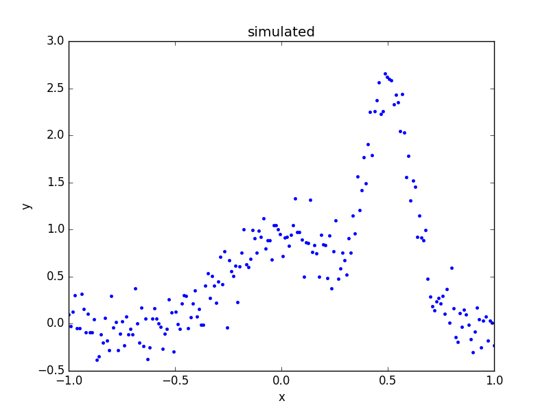
The model is evaluated on the grid, and “noise” added to it (using a normal distribution centered on 0 with a standard deviation of 0.2):
>>> x = np.linspace(-1, 1, 200)
>>> y = sim_model(x) + np.random.normal(0., 0.2, x.shape)
These arrays are placed into a Sherpa data object, using the
Data1D class, since it will be fit
below, and then a plot created to show the simulated data:
>>> d = data.Data1D('multiple', x, y)
>>> dplot = plot.DataPlot()
>>> dplot.prepare(d)
>>> dplot.plot()
What is the composite model?
The result of the combination is a
BinaryOpModel, which has
op,
lhs,
and rhs
attributes which describe the structure of the combination:
>>> sim_model
<BinaryOpModel model instance '(sim1 + sim2)'>
>>> sim_model.op
<ufunc 'add'>
>>> sim_model.lhs
<Gauss1D model instance 'sim1'>
>>> sim_model.rhs
<Gauss1D model instance 'sim2'>
There is also a
parts attribute
which contains all the elements of the model (in this case the
combination of the lhs and rhs attributes):
>>> sim_model.parts
(<Gauss1D model instance 'sim1'>, <Gauss1D model instance 'sim2'>)
>>> for cpt in sim_model.parts:
   ...:     print(cpt)
sim1
   Param        Type          Value          Min          Max      Units
   -----        ----          -----          ---          ---      -----
   sim1.fwhm    thawed          0.5  1.17549e-38  3.40282e+38
   sim1.pos     thawed            0 -3.40282e+38  3.40282e+38
   sim1.ampl    thawed            1 -3.40282e+38  3.40282e+38
sim2
   Param        Type          Value          Min          Max      Units
   -----        ----          -----          ---          ---      -----
   sim2.fwhm    thawed         0.25  1.17549e-38  3.40282e+38
   sim2.pos     thawed          0.5 -3.40282e+38  3.40282e+38
   sim2.ampl    thawed          2.5 -3.40282e+38  3.40282e+38
As the BinaryOpModel class is a subclass of the
ArithmeticModel class, the
combined model can be treated as a single model instance; for instance
it can be evaluated on a grid by passing in an array of values:
>>> sim_model([-1.0, 0, 1])
array([  1.52587891e-05,   1.00003815e+00,   5.34057617e-05])
Setting up the model
Rather than use the model components used to simulate the data, new instances are created and combined to create the model:
>>> g1 = models.Gauss1D('g1')
>>> g2 = models.Gauss1D('g2')
>>> mdl = g1 + g2
In this particular fit, the separation of the two models is going
to be assumed to be known, so the two pos parameters can
be linked together, which means that there
is one less free parameter in the fit:
>>> g2.pos = g1.pos + 0.5
The FWHM parameters are changed as the default value of 10 is not appropriate for this data (since the independent axis ranges from -1 to 1):
>>> g1.fwhm = 0.1
>>> g2.fwhm = 0.1
The display of the combined model shows that the g2.pos
parameter is now linked to the g1.pos value:
>>> print(mdl)
(g1 + g2)
   Param        Type          Value          Min          Max      Units
   -----        ----          -----          ---          ---      -----
   g1.fwhm      thawed          0.1  1.17549e-38  3.40282e+38
   g1.pos       thawed            0 -3.40282e+38  3.40282e+38
   g1.ampl      thawed            1 -3.40282e+38  3.40282e+38
   g2.fwhm      thawed          0.1  1.17549e-38  3.40282e+38
   g2.pos       linked          0.5     expr: (g1.pos + 0.5)
   g2.ampl      thawed            1 -3.40282e+38  3.40282e+38
Note
Good idea to check ranges (e.g. min/max) for parameters to make sure they are appropriate for the data.
The model is evaluated with its initial parameter values so that it can be compared to the best-fit location later:
>>> ystart = mdl(x)
Fitting the model
The initial model can be added to the data plot either directly,
with matplotlib commands, or using the
ModelPlot class to overlay onto the
DataPlot display:
>>> mplot = plot.ModelPlot()
>>> mplot.prepare(d, mdl)
>>> dplot.plot()
>>> mplot.plot(overplot=True)
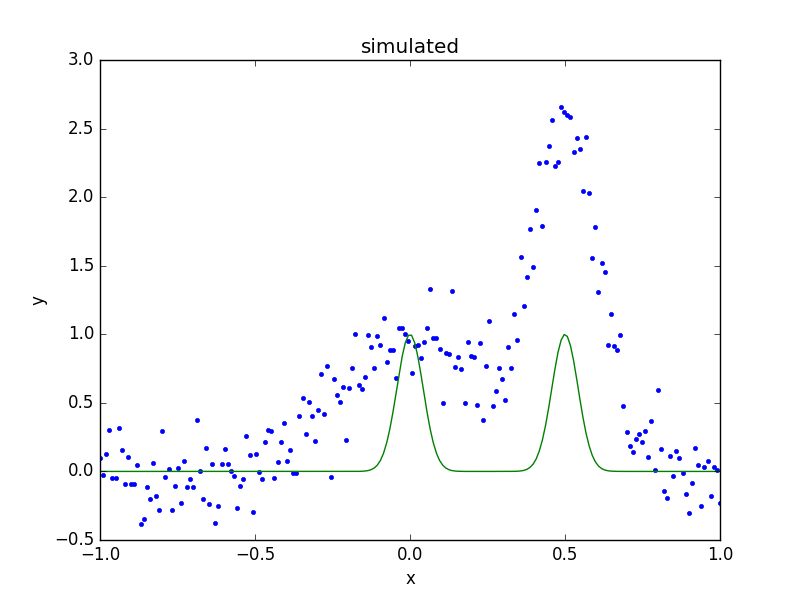
As can be seen, the initial values for the gaussian positions are close to optimal. This is unlikely to happen in real-world situations!
As there are no errors for the data set, the least-square statistic
(LeastSq) is used (so that
the fit attempts to minimise the separation between the model and
data with no weighting), along with the default optimiser:
>>> f = fit.Fit(d, mdl, stats.LeastSq())
>>> res = f.fit()
>>> res.succeeded
True
When displayig the results, the FitPlot
class is used since it combines both data and model plots (after
updating the mplot object to include the new model parameter
values):
>>> fplot = plot.FitPlot()
>>> mplot.prepare(d, mdl)
>>> fplot.prepare(dplot, mplot)
>>> fplot.plot()
>>> plt.plot(x, ystart, label='Start')
>>> plt.legend(loc=2)
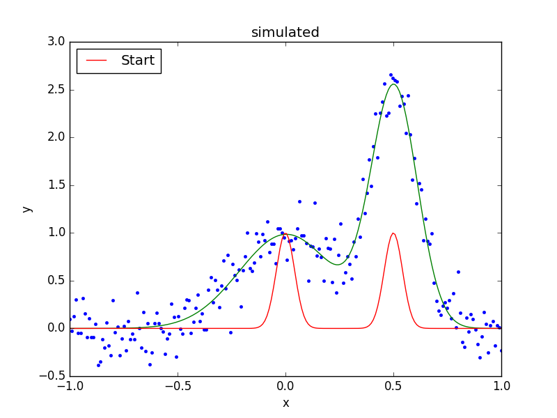
As can be seen below, the position of the g2 gaussian remains
linked to that of g1:
>>> print(mdl)
(g1 + g2)
   Param        Type          Value          Min          Max      Units
   -----        ----          -----          ---          ---      -----
   g1.fwhm      thawed     0.515565  1.17549e-38  3.40282e+38
   g1.pos       thawed   0.00431538 -3.40282e+38  3.40282e+38
   g1.ampl      thawed     0.985078 -3.40282e+38  3.40282e+38
   g2.fwhm      thawed     0.250698  1.17549e-38  3.40282e+38
   g2.pos       linked     0.504315     expr: (g1.pos + 0.5)
   g2.ampl      thawed      2.48416 -3.40282e+38  3.40282e+38
Accessing the linked parameter
The pars attribute of a model instance provides access to the
individual Parameter objects.
These can be used to query - as shown below - or change the model
values:
>>> for p in mdl.pars:
   ...:     if p.link is None:
   ...:         print("{:10s} -> {:.3f}".format(p.fullname, p.val))
   ...:     else:
   ...:         print("{:10s} -> link to {}".format(p.fullname, p.link.name))
g1.fwhm    -> 0.516
g1.pos     -> 0.004
g1.ampl    -> 0.985
g2.fwhm    -> 0.251
g2.pos     -> link to (g1.pos + 0.5)
g2.ampl    -> 2.484
The linked parameter is actually an instance of the
CompositeParameter
class, which allows parameters to be combined in a similar
manner to models:
>>> g2.pos
<Parameter 'pos' of model 'g2'>
>>> print(g2.pos)
val         = 0.504315379302
min         = -3.40282346639e+38
max         = 3.40282346639e+38
units       =
frozen      = True
link        = (g1.pos + 0.5)
default_val = 0.504315379302
default_min = -3.40282346639e+38
default_max = 3.40282346639e+38
>>> g2.pos.link
<BinaryOpParameter '(g1.pos + 0.5)'>
>>> print(g2.pos.link)
val         = 0.504315379302
min         = -3.40282346639e+38
max         = 3.40282346639e+38
units       =
frozen      = False
link        = None
default_val = 0.504315379302
default_min = -3.40282346639e+38
default_max = 3.40282346639e+38