Archive for the ‘Jargon’ Category.
Jul 25th, 2008| 01:12 pm | Posted by chasc
Diab Jerius follows up on LOESS techniques with a very nice summary update and finds LOCFIT to be very useful, but there are still questions about how it deals with measurement errors and combining observations from different experiments:
Continue reading ‘loess and lowess and locfit, oh my’ »
Tags:
Diab Jerius,
error,
experimental error,
local regression,
locfit,
Loess,
Lowess,
observational error,
Ping Zhao,
question for statisticians Category:
Algorithms,
Cross-Cultural,
Fitting,
Jargon,
Languages,
Stat,
Uncertainty |
2 Comments
Jul 23rd, 2008| 01:00 pm | Posted by vlk
With the LHC coming on line anon, it is appropriate to highlight the Banff Challenge, which was designed as a way to figure out how to place bounds on the mass of the Higgs boson. The equations that were to be solved are quite general, and are in fact the first attempt that I know of where calibration data are directly and explicitly included in the analysis. Continue reading ‘The Banff Challenge [Eqn]’ »
Jul 16th, 2008| 01:00 pm | Posted by vlk
The Χ2 distribution plays an incredibly important role in astronomical data analysis, but it is pretty much a black box to most astronomers. How many people know, for instance, that its form is exactly the same as the γ distribution? A Χ2 distribution with ν degrees of freedom is
p(z|ν) = (1/Γ(ν/2)) (1/2)ν/2 zν/2-1 e-z/2 ≡ γ(z;ν/2,1/2) , where z=Χ2.
Continue reading ‘chi-square distribution [Eqn]’ »
Jul 9th, 2008| 01:00 pm | Posted by vlk
The Kaplan-Meier (K-M) estimator is the non-parametric maximum likelihood estimator of the survival probability of items in a sample. “Survival” here is a historical holdover because this method was first developed to estimate patient survival chances in medicine, but in general it can be thought of as a form of cumulative probability. It is of great importance in astronomy because so much of our data are limited and this estimator provides an excellent way to estimate the fraction of objects that may be below (or above) certain flux levels. The application of K-M to astronomy was explored in depth in the mid-80′s by Jurgen Schmitt (1985, ApJ, 293, 178), Feigelson & Nelson (1985, ApJ 293, 192), and Isobe, Feigelson, & Nelson (1986, ApJ 306, 490). [See also Hyunsook's primer.] It has been coded up and is available for use as part of the ASURV package. Continue reading ‘Kaplan-Meier Estimator (Equation of the Week)’ »
Tags:
censored,
EotW,
Equation,
Equation of the Week,
Feigelson,
Isobe,
Kaplan-Meier,
maximum likelihood,
Nelson,
Schmitt,
survival analysis,
upper limit Category:
Frequentist,
Jargon,
Methods,
Stat |
13 Comments
Jul 2nd, 2008| 01:00 pm | Posted by vlk
Astrophysics, especially high-energy astrophysics, is all about counting photons. And this, it is said, naturally leads to all our data being generated by a Poisson process. True enough, but most astronomers don’t know exactly how it works out, so this derivation is for them. Continue reading ‘Poisson Likelihood [Equation of the Week]’ »
Jun 26th, 2008| 08:03 pm | Posted by hlee
What if R. A. Fisher was hired by the Royal Observatory in spite that his interest was biology and agriculture, or W. S. Gosset[] instead of brewery? An article by E.L. Lehmann made me think this what if. If so, astronomers could have handled errors better than now. Continue reading ‘On the history and use of some standard statistical models’ »
Jun 25th, 2008| 01:00 pm | Posted by vlk
For a discipline that relies so heavily on images, it is rather surprising how little use astronomy makes of the vast body of work on image analysis carried out by mathematicians and computer scientists. Mathematical morphology, for example, can be extremely useful in enhancing, recognizing, and extracting useful information from densely packed astronomical
images.
The building blocks of mathematical morphology are two operators, Erode[I|Y] and Dilate[I|Y], Continue reading ‘Open and Shut [Equation of the Week]’ »
Jun 19th, 2008| 11:42 pm | Posted by hlee
I was questioned by two attendees, acquainted before the AAS, if I can suggest them clustering methods relevant to their projects. After all, we spent quite a time to clarify the term clustering. Continue reading ‘my first AAS. IV. clustering’ »
Jun 18th, 2008| 01:00 pm | Posted by vlk
From Protassov et al. (2002, ApJ, 571, 545), here is a formal expression for the Likelihood Ratio Test Statistic,
TLRT = -2 ln R(D,Θ0,Θ)
R(D,Θ0,Θ) = [ supθεΘ0 p(D|Θ0) ] / [ supθεΘ p(D|Θ) ]
where D are an independent data sample, Θ are model parameters {θi, i=1,..M,M+1,..N}, and Θ0 form a subset of the model where θi = θi0, i=1..M are held fixed at their nominal values. That is, Θ represents the full model and Θ0 represents the simpler model, which is a subset of Θ. R(D,Θ0,Θ) is the ratio of the maximal (technically, supremal) likelihoods of the simpler model to that of the full model.
Continue reading ‘Likelihood Ratio Test Statistic [Equation of the Week]’ »
Tags:
EotW,
Equation,
Equation of the Week,
F-test,
likelihood,
likelihood ratio test,
LRT,
Protassov,
Rostislav Protassov Category:
Fitting,
Jargon,
Stat |
2 Comments
Jun 11th, 2008| 11:02 pm | Posted by hlee
Jun 11th, 2008| 01:00 pm | Posted by vlk
High-resolution astronomical spectroscopy has invariably been carried out with gratings. Even with the advent of the new calorimeter detectors, which can measure the energy of incoming photons to an accuracy of as low as 1 eV, gratings are still the preferred setups for hi-res work below energies of 1 keV or so. But how do they work? Where are the sources of uncertainty, statistical or systematic?
Continue reading ‘Grating Dispersion [Equation of the Week]’ »
Tags:
Bragg's Law,
Chandra,
diffraction,
dispersion,
EotW,
Equation,
Equation of the Week,
grating,
LETG,
Rowland Circle Category:
Astro,
Jargon,
Spectral |
2 Comments
Jun 8th, 2008| 08:38 pm | Posted by hlee
My first impression from the 212th AAS meeting is that it’s planned for preparing IYA 2009 and many talks are about current and future project reviews and strategies to reach public (People kept saying to me that winter meetings are more grand with expanded topics). I cannot say I understand everything (If someone says no astronomers understand everything, I’ll be relieved) but thanks to the theme of the meeting, I was intelligently entertained enough in many respects. The downside of this intellectual stimulus is growing doubts. One of those doubts was regression analysis in astronomy. Continue reading ‘my first AAS. I. Regression’ »
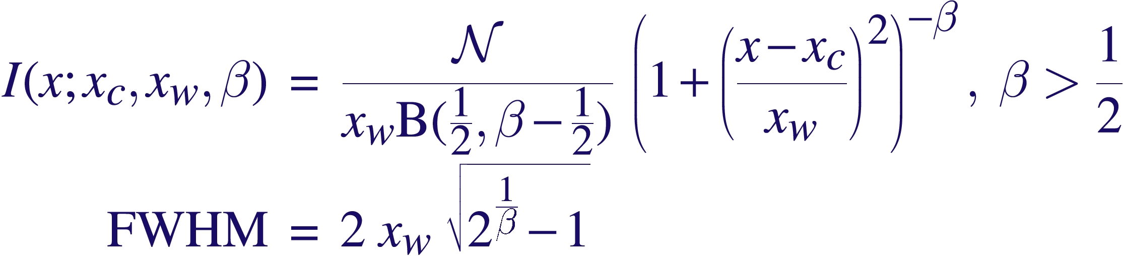
Jun 4th, 2008| 01:00 pm | Posted by vlk
X-ray telescopes generally work by reflecting photons at grazing incidence. As you can imagine, even small imperfections in the mirror polishing will show up as huge roadbumps to the incoming photons, and the higher their energy, the easier it is for them to scatter off their prescribed path. So X-ray telescopes tend to have sharp peaks and fat tails compared to the much more well-behaved normal-incidence telescopes, whose PSFs (Point Spread Functions) can be better approximated as Gaussians.
X-ray telescopes usually also have gratings that can be inserted into the light path, so that photons of different energies get dispersed by different angles, and whose actual energies can then be inferred accurately by measuring how far away on the detector they ended up. The accuracy of the inference is usually limited by the width of the PSF. Thus, a major contributor to the LRF (Line Response Function) is the aforementioned scattering.
A correct accounting of the spread of photons of course requires a full-fledged response matrix (RMF), but as it turns out, the line profiles can be fairly well approximated with Beta profiles, which are simply Lorentzians modified by taking them to the power β –
where B(1/2,β-1/2) is the Beta function, and N is a normalization constant defined such that integrating the Beta profile over the real line gives the area under the curve as N. The parameter β controls the sharpness of the function — the higher the β, the peakier it gets, and the more of it that gets pushed into the wings. Chandra LRFs are usually well-modeled with β~2.5, and XMM/RGS appears to require Lorentzians, β~1.
The form of the Lorentzian may also be familiar to people as the Cauchy Distribution, which you get for example when the ratio is taken of two quantities distributed as zero-centered Gaussians. Note that the mean and variance are undefined for that distribution.
Tags:
beta profile,
Chandra,
EotW,
Equation,
Equation of the Week,
Line Response Function,
Lorentzian,
LRF,
point spread function,
PSF,
response matrix,
RMF,
XMM Category:
Astro,
Jargon,
Misc |
1 Comment
May 28th, 2008| 01:00 pm | Posted by vlk
The most widely used tool for detecting sources in X-ray images, especially Chandra data, is the wavelet-based wavdetect, which uses the Mexican Hat (MH) wavelet. Now, the MH is not a very popular choice among wavelet aficianados because it does not form an orthonormal basis set (i.e., scale information is not well separated), and does not have compact support (i.e., the function extends to inifinity). So why is it used here?
Continue reading ‘Mexican Hat [EotW]’ »
Tags:
Chandra,
ciao,
convolution,
correlation,
EotW,
Equation,
Equation of the Week,
Fourier Transform,
gaussian,
MexHat,
Mexican Hat,
MH,
multiscale,
wavdetect,
wavelet Category:
Algorithms,
Astro,
Imaging,
Jargon |
1 Comment
May 21st, 2008| 01:00 pm | Posted by vlk
There is a lesson that statisticians, especially of the Bayesian persuasion, have been hammering into our skulls for ages: do not subtract background. Nevertheless, old habits die hard, and old codes die harder. Such is the case with X-ray aperture photometry. Continue reading ‘Background Subtraction [EotW]’ »
Tags:
aperture photometry,
background,
background marginalization,
background subtraction,
celldetect,
Chandra,
ciao,
EotW,
Equation,
error propagation,
ldetect,
local detect,
wavdetect,
X-ray Category:
Algorithms,
Astro,
Jargon |
6 Comments