Apr 30th, 2010| 12:12 pm | Posted by vlk
Sherpa is a fitting environment in which Chandra data (and really, X-ray data from any observatory) can be analyzed. It has just undergone a major update and now runs on python. Or allows python to run. Something like that. It is a very powerful tool, but I can never remember how to use it, and I have an amazing knack for not finding what I need in the documentation. So here is a little cheat sheet (which I will keep updating as and when if I learn more): Continue reading ‘Everybody needs crampons’ »
Tags:
Chandra,
cheat sheet,
ciao,
how to,
Python,
Sherpa,
Sherpa4 Category:
Algorithms,
Astro,
Fitting,
Jargon,
Languages |
2 Comments
Apr 2nd, 2009| 12:00 pm | Posted by hlee
I cannot remember when I first met Chernoff face but it hooked me up instantly. I always hoped for confronting multivariate data from astronomy applicable to this charming EDA method. Then, somewhat such eager faded, without realizing what’s happening. Tragically, this was mainly due to my absent mind. Continue reading ‘[MADS] Chernoff face’ »
Tags:
calibration,
Capella,
Chandra,
Chernoff face,
EDA,
line ratios,
MADS,
XAtlas Category:
Algorithms,
arXiv,
Astro,
Cross-Cultural,
Data Processing,
Jargon,
Methods,
Misc,
News,
Quotes,
Spectral,
Stars,
X-ray |
2 Comments
Nov 2nd, 2008| 08:42 am | Posted by vlk
Astronomy is known for its pretty pictures, but as Joe the Astronomer would say, those pretty pictures don’t make themselves. A lot of thought goes into maximizing scientific content while conveying just the right information, all discernible at a single glance. So the hardworkin folks at Chandra want your help in figuring out what works and how well, and they have set up a survey at http://astroart.cfa.harvard.edu/. Take the survey, it is both interesting and challenging!
Aug 27th, 2008| 07:50 am | Posted by vlk
UChicago, my alma mater, is doing alright for itself in the spacecraft naming business.
First there was Edwin Hubble (S.B. 1910, Ph.D. 1917).
Then came Arthur Compton (the “MetLab”).
Followed by Subramanya Chandrasekhar (Morton D. Hull Distinguished Service Professor of Theoretical Astrophysics).
And now, Enrico Fermi.
Tags:
CGRO,
Chandra,
Compton,
CXO,
Fermi,
GLAST,
HST,
Hubble,
observatory,
UChicago,
University of Chicago Category:
Astro,
gamma-ray,
High-Energy,
News,
Optical,
X-ray |
Comment
Jul 14th, 2008| 11:55 pm | Posted by vlk
Hyunsook recently said that she wished that there were “some astronomical data depositories where no data reduction is required but one can apply various statistical analyses to the data in the depository to learn and compare statistical methods”. With the caveat that there really is no such thing (every dataset will require case specific reduction; standard processing and reduction are inadequate in all but the simplest of cases), here is a brief list: Continue reading ‘Reduced and Processed Data’ »
Tags:
ADC,
astro catalogs,
Cast,
CDF-S,
Chandra,
datasets,
HEASARC,
Penn State,
reduced,
standard processing,
W3Browse Category:
Astro,
Data Processing,
Misc |
4 Comments
Jun 11th, 2008| 01:00 pm | Posted by vlk
High-resolution astronomical spectroscopy has invariably been carried out with gratings. Even with the advent of the new calorimeter detectors, which can measure the energy of incoming photons to an accuracy of as low as 1 eV, gratings are still the preferred setups for hi-res work below energies of 1 keV or so. But how do they work? Where are the sources of uncertainty, statistical or systematic?
Continue reading ‘Grating Dispersion [Equation of the Week]’ »
Tags:
Bragg's Law,
Chandra,
diffraction,
dispersion,
EotW,
Equation,
Equation of the Week,
grating,
LETG,
Rowland Circle Category:
Astro,
Jargon,
Spectral |
2 Comments
Jun 4th, 2008| 01:00 pm | Posted by vlk
X-ray telescopes generally work by reflecting photons at grazing incidence. As you can imagine, even small imperfections in the mirror polishing will show up as huge roadbumps to the incoming photons, and the higher their energy, the easier it is for them to scatter off their prescribed path. So X-ray telescopes tend to have sharp peaks and fat tails compared to the much more well-behaved normal-incidence telescopes, whose PSFs (Point Spread Functions) can be better approximated as Gaussians.
X-ray telescopes usually also have gratings that can be inserted into the light path, so that photons of different energies get dispersed by different angles, and whose actual energies can then be inferred accurately by measuring how far away on the detector they ended up. The accuracy of the inference is usually limited by the width of the PSF. Thus, a major contributor to the LRF (Line Response Function) is the aforementioned scattering.
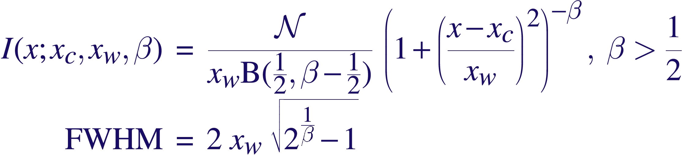
A correct accounting of the spread of photons of course requires a full-fledged response matrix (RMF), but as it turns out, the line profiles can be fairly well approximated with Beta profiles, which are simply Lorentzians modified by taking them to the power β –
where B(1/2,β-1/2) is the Beta function, and N is a normalization constant defined such that integrating the Beta profile over the real line gives the area under the curve as N. The parameter β controls the sharpness of the function — the higher the β, the peakier it gets, and the more of it that gets pushed into the wings. Chandra LRFs are usually well-modeled with β~2.5, and XMM/RGS appears to require Lorentzians, β~1.
The form of the Lorentzian may also be familiar to people as the Cauchy Distribution, which you get for example when the ratio is taken of two quantities distributed as zero-centered Gaussians. Note that the mean and variance are undefined for that distribution.
Tags:
beta profile,
Chandra,
EotW,
Equation,
Equation of the Week,
Line Response Function,
Lorentzian,
LRF,
point spread function,
PSF,
response matrix,
RMF,
XMM Category:
Astro,
Jargon,
Misc |
1 Comment
May 28th, 2008| 01:00 pm | Posted by vlk
The most widely used tool for detecting sources in X-ray images, especially Chandra data, is the wavelet-based wavdetect, which uses the Mexican Hat (MH) wavelet. Now, the MH is not a very popular choice among wavelet aficianados because it does not form an orthonormal basis set (i.e., scale information is not well separated), and does not have compact support (i.e., the function extends to inifinity). So why is it used here?
Continue reading ‘Mexican Hat [EotW]’ »
Tags:
Chandra,
ciao,
convolution,
correlation,
EotW,
Equation,
Equation of the Week,
Fourier Transform,
gaussian,
MexHat,
Mexican Hat,
MH,
multiscale,
wavdetect,
wavelet Category:
Algorithms,
Astro,
Imaging,
Jargon |
1 Comment
May 21st, 2008| 01:00 pm | Posted by vlk
There is a lesson that statisticians, especially of the Bayesian persuasion, have been hammering into our skulls for ages: do not subtract background. Nevertheless, old habits die hard, and old codes die harder. Such is the case with X-ray aperture photometry. Continue reading ‘Background Subtraction [EotW]’ »
Tags:
aperture photometry,
background,
background marginalization,
background subtraction,
celldetect,
Chandra,
ciao,
EotW,
Equation,
error propagation,
ldetect,
local detect,
wavdetect,
X-ray Category:
Algorithms,
Astro,
Jargon |
6 Comments
May 20th, 2008| 12:10 am | Posted by vlk
Earlier this year, Peter Edmonds showed me a press release that the Chandra folks were, at the time, considering putting out describing the possible identification of a Type Ia Supernova progenitor. What appeared to be an accreting white dwarf binary system could be discerned in 4-year old observations, coincident with the location of a supernova that went off in November 2007 (SN2007on). An amazing discovery, but there is a hitch.
And it is a statistical hitch, and involves two otherwise highly reliable and oft used methods giving contradictory answers at nearly the same significance level! Does this mean that the chances are actually 50-50? Really, we need a bona fide statistician to take a look and point out the errors of our ways.. Continue reading ‘Did they, or didn’t they?’ »
Tags:
arXiv,
Chandra,
CXC,
Optical,
Peter Edmonds,
positional coincidence,
positional error,
Power,
progenitor,
question for statisticians,
significance,
Supernova,
Type Ia,
White Dwarf,
White Dwarf binary,
X-ray Category:
arXiv,
Astro,
Data Processing,
News,
Objects,
Optical,
Stat,
Uncertainty |
5 Comments
Dec 14th, 2007| 05:53 pm | Posted by chasc
Our colleagues at Chandra public outreach have started a new blog, ChandraBlog – http://chandra.harvard.edu/blog/ which appears to be dedicated to news about the latest discoveries from Chandra. Mosey over and take a look.
Oct 21st, 2007| 03:59 pm | Posted by vlk
wavdetect is a wavelet-based source detection algorithm that is in wide use in X-ray data analysis, in particular to find sources in Chandra images. It came out of the Chicago “Beta Site” of the AXAF Science Center (what CXC used to be called before launch). Despite the fancy name, and the complicated mathematics and the devilish details, it is really not much more than a generalization of earlier local cell detect, where a local background is estimated around a putative source and the question is asked, is whatever signal that is being seen in this pixel significantly higher than expected? However, unlike previous methods that used a flux measurement as the criterion for detection (e.g., using signal-to-noise ratios as proxy for significance threshold), it tests the hypothesis that the observed signal can be obtained as a fluctuation from the background. Continue reading ‘The power of wavdetect’ »
Tags:
AXAF,
ChaMP,
Chandra,
ciao,
Power,
source detection,
Type II error,
wavdetect,
wavelet Category:
Algorithms,
Imaging,
X-ray |
1 Comment