gamma function (Equation of the Week)
The gamma function [not the Gamma -- note upper-case G -- which is related to the factorial] is one of those insanely useful functions that after one finds out about it, one wonders “why haven’t we been using this all the time?” It is defined only on the positive non-negative real line, is a highly flexible function that can emulate almost any kind of skewness in a distribution, and is a perfect complement to the Poisson likelihood. In fact, it is the conjugate prior to the Poisson likelihood, and is therefore a natural choice for a prior in all cases that start off with counts.
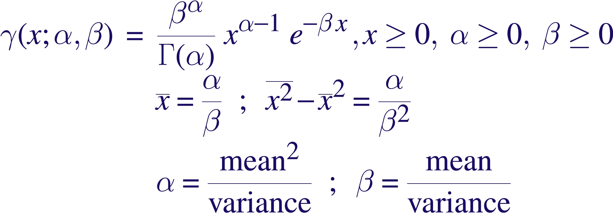
The gamma function is defined with two parameters, alpha, and beta, over the +ve non-negative real line. alpha can be any real number greater than 1 unlike the Poisson likelihood where the equivalent quantity are integers (values less than 1 are possible, but the function ceases to be integrable) and beta is any number greater than 0.
The mean is alpha/beta and the variance is alpha/beta2. Conversely, given a sample whose mean and variance are known, one can estimate alpha and beta to describe that sample with this function.
This is reminiscent of the Poisson distribution where alpha ~ number of counts and beta is akin to the collecting area or the exposure time. For this reason, a popular non-informative prior to use with the Poisson likelihood is gamma(alpha=1,beta=0), which is like saying “we expect to detect 0 counts in 0 time”. (Which, btw, is not the same as saying we detect 0 counts in an observation.) [Edit: see Tom Loredo's comments below for more on this.] Surprisingly, you can get less informative that even that, but that’s a discussion for another time.
Because it is the conjugate prior to the Poisson, it is also a useful choice to use as an informative prior. It makes derivations of formulae that much easier, though one has to be careful about using it blindly in real world applications, as the presence of background can muck up the pristine Poissonness of the prior (as we discovered while applying BEHR to Chandra Level3 products).
hlee:
In an introductory stat class, I taught for engineers briefly, to give them a practical sense of this gamma density function, I gave them the following example: There are α bags and each bag contains the same type of radio active stones collected from one region but different batches of land. A decay rate (1/β) is important to understand the oldness of the excavation region (ignoring testing samples in bags are homogeneous or not). If there’s one bag of stones, then it is an exponential density function or a Poisson pmf. Based on sample stones from α (known at this point) bags, I’d like to estimate 1/β from the stones in α bags.
I’m not sure if the above example is proper or not. Normal text books stop providing examples at Poisson or the exponential. Until graduate textbooks, no one would care the gamma density function is one of density functions, let alone it’s a conjugate prior of Poisson. Unless one is dealing with a Poisson likelihood and considering computing a posterior (astronomy posteriors require heavy computations in general), the gamma density function does not receive its spot light often. When I saw the title γ function, the first impression was Γ(x)=(x-1)!
05-07-2008, 3:03 pmTomLoredo:
A terminological quibble: it’s the gamma distribution that you are discussing here, not the gamma function (which appears in the distribution’s normalization constant). Either formula is a good choice for EotW, and you gave a good capsule description of the distribution. Wikipedia has a good entry on the gamma distribution for those who would like to learn more: Gamma Distribution. (BTW, Wikipedia’s entries on common distributions tend to be of pretty high quality in my experience.)
Besides being the conjugate prior for the rate (or mean number of counts) of a constant Poisson counting process, the gamma distribution with argument (1/x) rather than x, dubbed the inverse gamma distribution for x, is the conjugate prior for the variance of a normal (Gaussian) distribution.
My further quibble is with the remark that the gamma(alpha=1,beta=0) prior “is like saying ‘we expect to detect 0 counts in 0 time’.” What prior (gamma or otherwise) that does not put all its probability at infinity does not say “we expect to detect 0 counts in 0 time?” This is a basic property of the Poisson distribution: the expected number of counts is proportional to the interval size (for any finite rate), so no matter what you say about the rate (a priori or a posteriori), you expect 0 events in an interval of 0 measure.
Here’s one way to look at what the gamma(alpha=1,beta=0) prior says: the probability I assign to seeing n counts in any particular interval of nonzero size is independent of n; that is, the prior expresses no preference for the number of counts expected a priori. I suppose this must be in the literature somewhere. I noted this justification for the flat (in x) prior back in my 1992 paper for the 1st SCMA conference. I’m not sure it made the printed version (which was highly abridged from the submitted one), but the long version is online: The Promise of Bayesian Inference for Astrophysics. The argument is on pp. 42-43, and makes use of the fact that an integral over a gamma distribution can be interpreted as a Laplace transform.
I stole this argument from Thomas Bayes. It is analogous to his justification for a flat prior for the single-trial probability parameter in a binomial distribution. He argued for a flat prior, not by arguing that uniformity of the prior density was in some sense a natural expression of “ignorance” (as is often attributed to him) but rather that uniformity of the predictive distribution for the number of successes was a useful description of ignorance. (See Stephen Stigler’s paper on Bayes’s famous paper for discussion of the misunderstanding of Bayes’s reasoning.)
A virtue of these predictive criteria for non-informative priors is that they are immune to the usual complaint that flatness of a prior for a parameter is parameterization-dependent. Of course, one could argue about “reparameterizing” the sample space. In these problems, with discrete sample spaces, such arguments seem more than a bit of a stretch. Unfortunately, I think such predictive arguments are only feasible for fairly simple problems. But some of those simple problems are important—like this one!
05-07-2008, 5:44 pmvlk:
Thanks, Tom, for a very illuminating comment!
You are right of course that we use it mostly as a distribution, and indeed, the second line in the equation cannot apply to anything else. But I wanted to highlight the fact that it really is also a function, and can be used as such. Quite often we come across quantities that are defined on the +ve line, but people continue to use Gaussians to fit to them when in fact a gamma function would be more desirable.
I am confused though about priors putting probability at infinity always being equivalent to 0 counts in 0 time. The nice thing about alpha=1,beta=0 is that it is exactly like a Poisson likelihood for such an “observation”, and contrarily, there are other improper priors which go off to infinity but don’t have that nice correspondence with the Poisson likelihood (alpha=0.5, for instance, which apparently is the Fisher least information prior, or to take a completely different function, the Lorentzian). What is the difference between these cases then?
05-08-2008, 9:52 pmTomLoredo:
Hi Vinay-
But I wanted to highlight the fact that it really is also a function, and can be used as such. Quite often we come across quantities that are defined on the +ve line, but people continue to use Gaussians to fit to them when in fact a gamma function would be more desirable.
(Note it’s defined on the non-negative real line, not just +ve; it’s important that it includes zero.)
Can you give an example where it appears in astronomy as a function and not a distribution? Your example has it as a distribution. The only thing close to this that I can think is fitting unnormalized number counts, where one could use a function proportional to a gamma distribution as the intensity for an inhomogeneous point process (a Schechter function is in this vein). But in this case it’s still a distribution, albeit a measure that may not be normalized to unit area (a Poisson process intensity is a measure).
In any case, “gamma function” is already the name for \Gamma(x) (in TeX notation), the function that equals n! when x=n+1 for a nonnegative integer n. Both lower and upper case “gamma” (the word, not the symbol) are used for this in the literature (e.g., Numerical Recipes and the various Wolfram products, including Mathematica, use the lower case), so maybe you need to come up with a different name if you want to distinguish the functional form from the distribution. And in that case, you might as well drop the normalization constants. I have seen authors use “Gaussian” for any function proportional to exp(-x**2) (for appropriate x), and reserve “normal distribution” for the normalized form (including the sqrt(2pi), etc.). Perhaps we need to come up with a similar separate name for the functional form underlying the gamma distribution. Maybe just “truncated power law” or “exponentially truncated power law.”
Regarding the prior, I did not write that “priors putting [all] probability at infinity [are] equivalent to 0 counts in 0 time;” that’s nearly the opposite of what I wrote. Referring to your original statement that the (1,0) prior means “we expect to detect 0 counts in 0 time,” I stated that any prior that does not put all its mass at infinity says we expect to detect 0 counts in 0 time, since for any finite rate, the Poisson distribution for an interval of zero size puts all the probability at n=0 (“we expect to detect 0 counts in 0 time). So your statement cannot be a sound justification for the (1,0) prior. Sorry for the confusion; perhaps it’s clearer now.
Also, note that the gamma distribution is only defined for beta>0, so (1,0) is not a legitimate gamma distribution. This is where it’s useful to distinguish the distribution from the functional form (and perhaps was part of your motivation in doing so). The (1,0) limit of the distribution’s functional form (including the normalization constants in your definition) is 0, which isn’t a very good prior for anything. The (1,0) limit of the functional form without the normalization factors is a constant, and thus cannot be used as a probability distribution over the non-negative real line (in Bayesian language, it would be an improper prior). In other words, a flat prior is not a gamma distribution, though it is a special case of an “exponentially truncated power law.”
05-12-2008, 3:59 pmhlee:
I have a bit fundamental issue (asking for correction) to address after reading your comments. There seems to be a mix between fitting and modeling. Fitting includes finding best fit parameters based on a given source model and depending on assumptions on an error structure or distance metrics, error bars can be obtained (most cases, least square fitting based on the L_2 norm, equivalent to the gaussian errors). Here error estimates are by-products of fitting process and if the metric changes the error changes. The other is modeling, focusing on estimating the distribution of errors. Not necessarily because of nonparametric methods, but particularly in Bayesian analysis, one has to assume a parametric distribution where fitting techniques are often used. Since it is modeling process, the uncertainty measure from this parametric distribution is the error we are interested in. I hope readers of your comments would consider the directional differences between fitting and modeling.
05-12-2008, 10:24 pmvlk:
“Can you give an example where it appears in astronomy as a function and not a distribution?”
Afraid not, Tom. Because even when such an “exponentially truncated power-law” might have been the appropriate function, people have used Gaussians instead.
So yes, I do mean fitting, with an honest-to-goodness function, the same way one might fit a spectral line with a Gaussian. Essentially to any quantity that does not extend to the -ve line. Such as the radial profile of a piled-up PSF to come up with a contrived example. I can give you a case where _I_ ought to have resorted to fitting with the gamma but didn’t — e.g., see Fig 8 of Chung et al. (2004, ApJ, 606, 1184). I will keep an eye peeled out for other cases to highlight.
Hyunsook, I don’t understand the distinction you make between fitting and modeling. It could be you are referring to some statistics-only definition of what a “model” means? In any case, I don’t see how error-estimates are dependent on the fitting _process_.
05-12-2008, 11:00 pmvlk:
PS: OK, yes Hyunsook, I guess I have seen cases where the estimated error is dependent on the choice of the fitting method. The Banff Challenge being a glaring example. Is that what you meant?
PPS: Tom, I forgot we did indeed use the gamma quite recently. Given the posterior draws of a Poisson intensity obtained with BEHR, we fit (yea, fit) a gamma function to the sample to determine the parameters of the prior going forward to the next observation. You could rightly say that it is being used as a distribution, but for a tiny step in there after the sampling and before being set as the prior, it was indeed used as a function.
05-13-2008, 12:06 pmhlee:
From the modeling point of view, your γ function cannot be a legitimate density function if you allow β=0. From the fitting point of view, the constraints on α and β are not necessarily unless physics specifies them, and so it’s only a (alleged- if there’s another definition under the same name) gamma function. Still it’s not a density function to describe the error distribution. I just wanted to point out that the same object can be used for fitting and modeling but should stay within the dogma. Although disappointment is expected from some subscribers, I rather not walk through all the details via Banff challenge about how error estimates change depending on fitting methods. The story can be extended to post model selection, testing misspecified models (F test and LRT stuffs), and overall statistics, obviously beyond my reach.
05-14-2008, 4:53 pm