Data Tables (`astropy.table`)¶

Introduction¶

astropy.table provides functionality for storing and manipulating heterogeneous tables of data in a way that is familiar to numpy users. A few notable capabilities of this package are:

Initialize a table from a wide variety of input data structures and types.
Modify a table by adding or removing columns, changing column names, or adding new rows of data.
Handle tables containing missing values.
Include table and column metadata as flexible data structures.
Specify a description, units and output formatting for columns.
Interactively scroll through long tables similar to using more.
Create a new table by selecting rows or columns from a table.
Perform Table operations like database joins, concatenation, and binning.
Maintain a table index for fast retrieval of table items or ranges.
Manipulate multidimensional columns.
Handle non-native (mixin) column types within table.
Methods for Reading and writing Table objects to files.
Hooks for Subclassing Table and its component classes.

Getting Started¶

The basic workflow for creating a table, accessing table elements, and modifying the table is shown below. These examples show a very simple case, while the full astropy.table documentation is available from the Using table section.

First create a simple table with columns of data named a, b, c, and d. These columns have integer, float, string, and Quantity values respectively:

>>> from astropy.table import QTable
>>> import astropy.units as u
>>> a = [1, 4, 5]
>>> b = [2.0, 5.0, 8.2]
>>> c = ['x', 'y', 'z']
>>> d = [10, 20, 30] * u.m / u.s
>>> t = QTable([a, b, c, d],
...            names=('a', 'b', 'c', 'd'),
...            meta={'name': 'first table'})

Notice the use of a Quantity array for column d. Since we used QTable this stores a native Quantity within the table and brings the full power of Units and Quantities (astropy.units) to this column in the table.

Note

If the table data have no units or you prefer to not use Quantity then you can use the Table class to create tables. The only difference between QTable and Table is the behavior when adding a column that has units. See Quantity and QTable and Columns with Units for details on the differences and use cases.

There are many other ways to construct a table, including from a list of rows (either tuples or dicts), from a numpy structured or 2-d array, by adding columns or rows incrementally, or even from a pandas pandas.DataFrame. See Constructing a table for the details.

There are a few ways to examine the table. You can get detailed information about the table values and column definitions as follows:

>>> t
<QTable length=3>
  a      b      c       d
                      m / s
int32 float64 bytes1 float64
----- ------- ------ -------
    1     2.0      x    10.0
    4     5.0      y    20.0
    5     8.2      z    30.0

Finally, you can get summary information about the table as follows:

>>> t.info
<QTable length=3>
name  dtype   unit  class
---- ------- ----- --------
   a   int32         Column
   b float64         Column
   c  bytes1         Column
   d float64 m / s Quantity

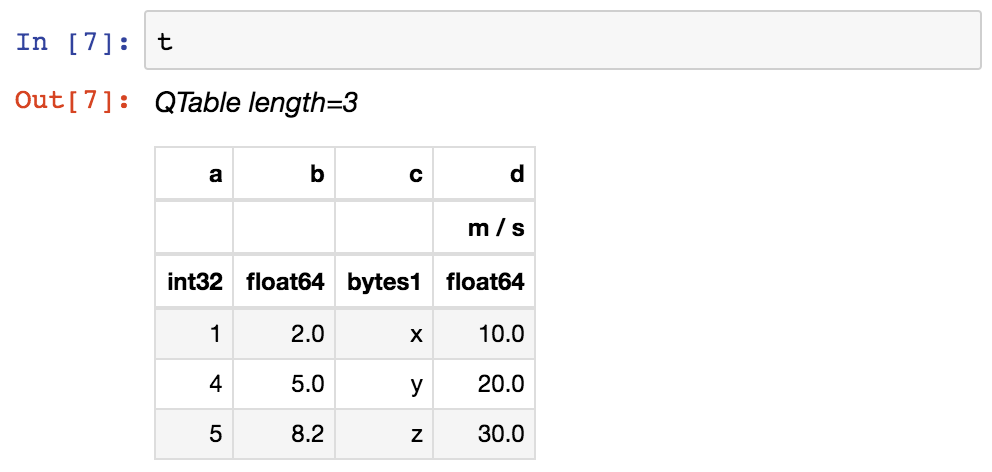
From within a Jupyter notebook, the table is displayed as a formatted HTML table (details of how it appears can be changed by altering the astropy.table.default_notebook_table_class configuration item):

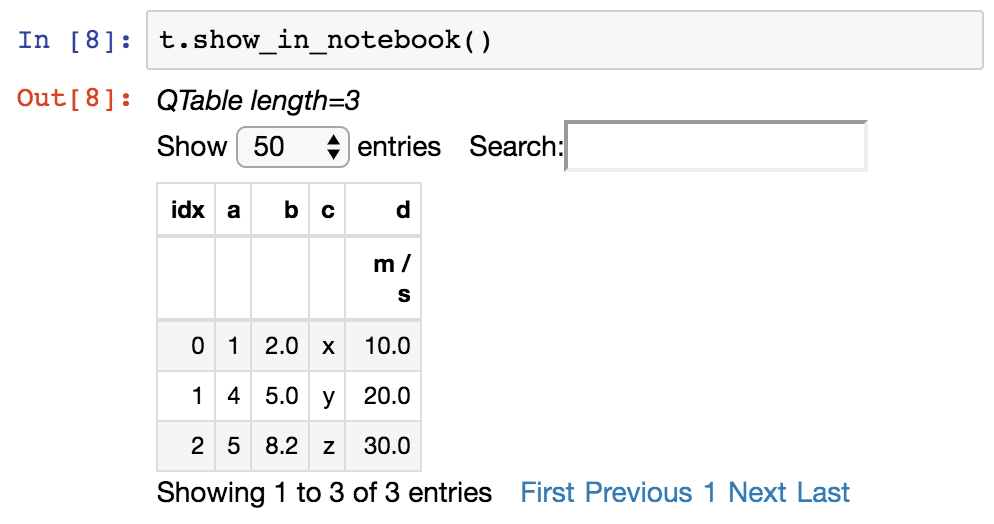
Or you can get a fancier notebook interface with in-browser search and sort using show_in_notebook:

If you print the table (either from the notebook or in a text console session) then a formatted version appears:

>>> print(t)
 a   b   c    d
            m / s
--- --- --- -----
  1 2.0   x  10.0
  4 5.0   y  20.0
  5 8.2   z  30.0

If you do not like the format of a particular column, you can change it:

>>> t['b'].info.format = '7.3f'
>>> print(t)
 a     b     c    d
                m / s
--- ------- --- -----
  1   2.000   x  10.0
  4   5.000   y  20.0
  5   8.200   z  30.0

For a long table you can scroll up and down through the table one page at time:

>>> t.more()  

You can also display it as an HTML-formatted table in the browser:

>>> t.show_in_browser()  

or as an interactive (searchable & sortable) javascript table:

>>> t.show_in_browser(jsviewer=True)  

Now examine some high-level information about the table:

>>> t.colnames
['a', 'b', 'c', 'd']
>>> len(t)
3
>>> t.meta
{'name': 'first table'}

Access the data by column or row using familiar numpy structured array syntax:

>>> t['a']       # Column 'a'
<Column name='a' dtype='int32' length=3>
1
4
5

>>> t['a'][1]    # Row 1 of column 'a'
4

>>> t[1]         # Row object for table row index=1
<Row index=1>
  a      b      c       d
                      m / s
int32 float64 bytes1 float64
----- ------- ------ -------
    4   5.000      y    20.0


>>> t[1]['a']    # Column 'a' of row 1
4

You can retrieve a subset of a table by rows (using a slice) or columns (using column names), where the subset is returned as a new table:

>>> print(t[0:2])      # Table object with rows 0 and 1
 a     b     c    d
                m / s
--- ------- --- -----
  1   2.000   x  10.0
  4   5.000   y  20.0


>>> print(t['a', 'c'])  # Table with cols 'a', 'c'
 a   c
--- ---
  1   x
  4   y
  5   z

Modifying table values in place is flexible and works as one would expect:

>>> t['a'][:] = [-1, -2, -3]    # Set all column values in place
>>> t['a'][2] = 30              # Set row 2 of column 'a'
>>> t[1] = (8, 9.0, "W", 4 * u.m / u.s) # Set all row values
>>> t[1]['b'] = -9              # Set column 'b' of row 1
>>> t[0:2]['b'] = 100.0         # Set column 'b' of rows 0 and 1
>>> print(t)
 a     b     c    d
                m / s
--- ------- --- -----
 -1 100.000   x  10.0
  8 100.000   W   4.0
 30   8.200   z  30.0

Replace, add, remove, and rename columns with the following:

>>> t['b'] = ['a', 'new', 'dtype']   # Replace column b (different from in-place)
>>> t['e'] = [1, 2, 3]               # Add column d
>>> del t['c']                       # Delete column c
>>> t.rename_column('a', 'A')        # Rename column a to A
>>> t.colnames
['A', 'b', 'd', 'e']

Adding a new row of data to the table is as follows. Note that the unit value is given in cm / s but will be added to the table as 0.1 m / s in accord with the existing unit.

>>> t.add_row([-8, -9, 10 * u.cm / u.s, 11])
>>> len(t)
4

You can create a table with support for missing values, for example by setting masked=True:

>>> t = QTable([a, b, c], names=('a', 'b', 'c'), masked=True, dtype=('i4', 'f8', 'U1'))
>>> t['a'].mask = [True, True, False]
>>> t
<QTable masked=True length=3>
  a      b     c
int32 float64 str1
----- ------- ----
   --     2.0    x
   --     5.0    y
    5     8.2    z

In addition to Quantity, you can include certain object types like Time, SkyCoord, and NdarrayMixin in your table. These “mixin” columns behave like a hybrid of a regular Column and the native object type (see Mixin columns). For example:

>>> from astropy.time import Time
>>> from astropy.coordinates import SkyCoord
>>> tm = Time(['2000:002', '2002:345'])
>>> sc = SkyCoord([10, 20], [-45, +40], unit='deg')
>>> t = QTable([tm, sc], names=['time', 'skycoord'])
>>> t
<QTable length=2>
         time          skycoord
                       deg,deg
        object          object
--------------------- ----------
2000:002:00:00:00.000 10.0,-45.0
2002:345:00:00:00.000  20.0,40.0

Using `table`¶

The details of using astropy.table are provided in the following sections:

I/O with tables¶

Mixin columns¶

Mixin columns

Implementation¶

Table implementation details

Performance Tips¶

Constructing Table objects row-by-row using add_row() can be very slow:

>>> from astropy.table import Table
>>> t = Table(names=['a', 'b'])
>>> for i in range(100):
...    t.add_row((1, 2))

If you do need to loop in your code to create the rows, a much faster approach is to construct a list of rows and then create the Table object at the very end:

>>> rows = []
>>> for i in range(100):
...    rows.append((1, 2))
>>> t = Table(rows=rows, names=['a', 'b'])

Writing a Table with MaskedColumn to .ecsv using write() can be very slow:

>>> from astropy.table import Table
>>> import numpy as np
>>> x = np.arange(10000, dtype=float)
>>> tm = Table([x], masked=True)
>>> tm.write('tm.ecsv', overwrite=True) 

If you want to write .ecsv using write(), then use serialize_method='data_mask'. It uses the non-masked version of data and it is faster:

>>> tm.write('tm.ecsv', overwrite=True, serialize_method='data_mask') 

Reference/API¶

astropy.table Package¶

Functions¶

`cstack`(tables[, join_type, metadata_conflicts])	Stack columns within tables depth-wise
`hstack`(tables[, join_type, uniq_col_name, …])	Stack tables along columns (horizontally)
`join`(left, right[, keys, join_type, …])	Perform a join of the left table with the right table on specified keys.
`represent_mixins_as_columns`(tbl[, …])	Represent input Table `tbl` using only `Column` or `MaskedColumn` objects.
`setdiff`(table1, table2[, keys])	Take a set difference of table rows.
`unique`(input_table[, keys, silent, keep])	Returns the unique rows of a table.
`vstack`(tables[, join_type, metadata_conflicts])	Stack tables vertically (along rows)

Classes¶

`BST`(data, row_index[, unique])	A basic binary search tree in pure Python, used as an engine for indexing.
`Column`	Define a data column for use in a Table object.
`ColumnGroups`(parent_column[, indices, keys])
`ColumnInfo`([bound])	Container for meta information like name, description, format.
`Conf`	Configuration parameters for `astropy.table`.
`FastBST`	alias of `astropy.table.BST`
`FastRBT`	alias of `astropy.table.BST`
`JSViewer`([use_local_files, display_length])	Provides an interactive HTML export of a Table.
`MaskedColumn`	Define a masked data column for use in a Table object.
`NdarrayMixin`	Mixin column class to allow storage of arbitrary numpy ndarrays within a Table.
`QTable`([data, masked, names, dtype, meta, …])	A class to represent tables of heterogeneous data.
`Row`(table, index)	A class to represent one row of a Table object.
`SCEngine`(data, row_index[, unique])	Fast tree-based implementation for indexing, using the `sortedcontainers` package.
`SerializedColumn`	Subclass of dict that is a used in the representation to contain the name (and possible other info) for a mixin attribute (either primary data or an array-like attribute) that is serialized as a column in the table.
`SortedArray`(data, row_index[, unique])	Implements a sorted array container using a list of numpy arrays.
`StringTruncateWarning`	Warning class for when a string column is assigned a value that gets truncated because the base (numpy) string length is too short.
`Table`([data, masked, names, dtype, meta, …])	A class to represent tables of heterogeneous data.
`TableColumns`([cols])	OrderedDict subclass for a set of columns.
`TableFormatter`
`TableGroups`(parent_table[, indices, keys])
`TableMergeError`
`TableReplaceWarning`	Warning class for cases when a table column is replaced via the Table.__setitem__ syntax e.g.

Data Tables (`astropy.table`)¶

Introduction¶

Getting Started¶

Using `table`¶

Construct table¶

Access table¶

Modify table¶

Table operations¶

Indexing¶

Masking¶

I/O with tables¶

Mixin columns¶

Implementation¶

Performance Tips¶

Reference/API¶

astropy.table Package¶

Functions¶

Classes¶

Class Inheritance Diagram¶

Page Contents

Navigation

Data Tables (astropy.table)¶

Introduction¶

Getting Started¶

Using table¶

Construct table¶

Access table¶

Modify table¶

Table operations¶

Indexing¶

Masking¶

I/O with tables¶

Mixin columns¶

Implementation¶

Performance Tips¶

Reference/API¶

astropy.table Package¶

Functions¶

Classes¶

Class Inheritance Diagram¶

Data Tables (`astropy.table`)¶

Using `table`¶