The AstroStat Slog

Now it’s time for me to write my own astrostat papers instead of spending time for sieving them from [arXiv]. It has been an irresistible temptation scanning daily [arXiv] preprints to look for astronomy and sometimes statistics papers that 1. adopt statistics, 2. contain statistically challenging problems, 3. could be improved by more rigorous statistical applications, 4. look like abusing statistics, 5. may inspire statisticians by the data sets, or 6. might be useful for astronomers’ advancement in the data analysis. The temptation grew too much to be handled. The amount of papers belong to the above selection criteria seems to grow as my understanding widens. Also the mesh gets loose and starts to show holes. …Continue reading»

This is my last [ArXiv] series. …Continue reading»

One realization of mine during the meeting was related to a cultural difference; therefore, there is no relation to any presentations during the 212th AAS in this post. Please, correct me if you find wrong statements. I cannot cover all perspectives from both disciplines but I think there are two distinct fashions in practicing normalization. …Continue reading»

What is systematic error? Can it be modeled statistically? Is it random? Is it fixed? Is it a bias? Is it …? …Continue reading»

While discussing different view points on the term, clustering, one of the conversers led me to his colleague’s poster. This poster (I don’t remember its title and abstract) was my favorite from all posters in the meeting. …Continue reading»

I was questioned by two attendees, acquainted before the AAS, if I can suggest them clustering methods relevant to their projects. After all, we spent quite a time to clarify the term clustering. …Continue reading»

You all may have heard that GLAST launched on June 11, and the mission is going smoothly. Via Josh Grindlay comes news that Steve Ritz, the GLAST Project Scientist at GSFC, is keeping a weblog dedicated to it at

http://blogs.nasa.gov/cm/blog/GLAST

and intends to post status reports and related information on it.

From Protassov et al. (2002, ApJ, 571, 545), here is a formal expression for the Likelihood Ratio Test Statistic,

T_LRT = -2 ln R(D,Θ₀,Θ)

R(D,Θ₀,Θ) = [ sup_θεΘ0 p(D|Θ₀) ] / [ sup_θεΘ p(D|Θ) ]

where D are an independent data sample, Θ are model parameters {θ_i, i=1,..M,M+1,..N}, and Θ₀ form a subset of the model where θ_i = θ_i⁰, i=1..M are held fixed at their nominal values. That is, Θ represents the full model and Θ₀ represents the simpler model, which is a subset of Θ. R(D,Θ₀,Θ) is the ratio of the maximal (technically, supremal) likelihoods of the simpler model to that of the full model.
…Continue reading»

As Prof. Speed said, PCA is prevalent in astronomy, particularly this week. Furthermore, a paper explicitly discusses R, a popular statistics package. …Continue reading»

Believe it or not, I saw ANOVA (ANalysis Of VAriance) from a poster at AAS. This acronym was considered as one of very statistical jargons that one would never see in an astronomical meeting. I think you like to know the story in detail. …Continue reading»

What is the maximum likelihood test in astronomy? …Continue reading»

High-resolution astronomical spectroscopy has invariably been carried out with gratings. Even with the advent of the new calorimeter detectors, which can measure the energy of incoming photons to an accuracy of as low as 1 eV, gratings are still the preferred setups for hi-res work below energies of 1 keV or so. But how do they work? Where are the sources of uncertainty, statistical or systematic?
…Continue reading»

Despite no statistic related discussion, a paper comparing XSPEC and ISIS, spectral analysis open source applications might bring high energy astrophysicists’ interests this week. …Continue reading»

My first impression from the 212th AAS meeting is that it’s planned for preparing IYA 2009 and many talks are about current and future project reviews and strategies to reach public (People kept saying to me that winter meetings are more grand with expanded topics). I cannot say I understand everything (If someone says no astronomers understand everything, I’ll be relieved) but thanks to the theme of the meeting, I was intelligently entertained enough in many respects. The downside of this intellectual stimulus is growing doubts. One of those doubts was regression analysis in astronomy. …Continue reading»

X-ray telescopes generally work by reflecting photons at grazing incidence. As you can imagine, even small imperfections in the mirror polishing will show up as huge roadbumps to the incoming photons, and the higher their energy, the easier it is for them to scatter off their prescribed path. So X-ray telescopes tend to have sharp peaks and fat tails compared to the much more well-behaved normal-incidence telescopes, whose PSFs (Point Spread Functions) can be better approximated as Gaussians.

X-ray telescopes usually also have gratings that can be inserted into the light path, so that photons of different energies get dispersed by different angles, and whose actual energies can then be inferred accurately by measuring how far away on the detector they ended up. The accuracy of the inference is usually limited by the width of the PSF. Thus, a major contributor to the LRF (Line Response Function) is the aforementioned scattering.

A correct accounting of the spread of photons of course requires a full-fledged response matrix (RMF), but as it turns out, the line profiles can be fairly well approximated with Beta profiles, which are simply Lorentzians modified by taking them to the power β –

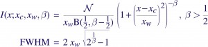
where B(1/2,β-1/2) is the Beta function, and N is a normalization constant defined such that integrating the Beta profile over the real line gives the area under the curve as N. The parameter β controls the sharpness of the function — the higher the β, the peakier it gets, and the more of it that gets pushed into the wings. Chandra LRFs are usually well-modeled with β~2.5, and XMM/RGS appears to require Lorentzians, β~1.

The form of the Lorentzian may also be familiar to people as the Cauchy Distribution, which you get for example when the ratio is taken of two quantities distributed as zero-centered Gaussians. Note that the mean and variance are undefined for that distribution.