The AstroStat Slog

So far, I didn’t complain much related to my “statistician learning astronomy” experience. Instead, I’ve been trying to emphasize how fascinating it is. I hope that more statisticians can join this adventure when statisticians’ insights are on demand more than ever. However, this positivity seems not working so far. In two years of this slog’s life, there’s no posting by a statistician, except one about BEHR. Statisticians are busy and well distracted by other fields with more tangible data sets. Or compared to other fields, too many obstacles and too high barriers exist in astronomy for statisticians to participate. I’d like to talk about these challenges from my ends.^[1] Continue reading ‘data analysis system and its documentation’ »

1. This is quite an overdue posting. Links and associated content can be outdated.[↩]

RMF. It is a wørd to strike terror even into the hearts of the intrepid. It refers to the spread in the measured energy of an incoming photon, and even astronomers often stumble over what it is and what it contains. It essentially sets down the measurement error for registering the energy of a photon in the given instrument.

Thankfully, its usage is robustly built into analysis software such as Sherpa or XSPEC and most people don’t have to deal with the nitty gritty on a daily basis. But given the profusion of statistical software being written for astronomers, it is perhaps useful to go over what it means. Continue reading ‘Redistribution’ »

X-ray telescopes generally work by reflecting photons at grazing incidence. As you can imagine, even small imperfections in the mirror polishing will show up as huge roadbumps to the incoming photons, and the higher their energy, the easier it is for them to scatter off their prescribed path. So X-ray telescopes tend to have sharp peaks and fat tails compared to the much more well-behaved normal-incidence telescopes, whose PSFs (Point Spread Functions) can be better approximated as Gaussians.

X-ray telescopes usually also have gratings that can be inserted into the light path, so that photons of different energies get dispersed by different angles, and whose actual energies can then be inferred accurately by measuring how far away on the detector they ended up. The accuracy of the inference is usually limited by the width of the PSF. Thus, a major contributor to the LRF (Line Response Function) is the aforementioned scattering.

A correct accounting of the spread of photons of course requires a full-fledged response matrix (RMF), but as it turns out, the line profiles can be fairly well approximated with Beta profiles, which are simply Lorentzians modified by taking them to the power β –

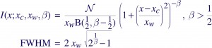
where B(1/2,β-1/2) is the Beta function, and N is a normalization constant defined such that integrating the Beta profile over the real line gives the area under the curve as N. The parameter β controls the sharpness of the function — the higher the β, the peakier it gets, and the more of it that gets pushed into the wings. Chandra LRFs are usually well-modeled with β~2.5, and XMM/RGS appears to require Lorentzians, β~1.

The form of the Lorentzian may also be familiar to people as the Cauchy Distribution, which you get for example when the ratio is taken of two quantities distributed as zero-centered Gaussians. Note that the mean and variance are undefined for that distribution.

Starting a new feature — highlighting some equation that is widely used in astrophysics or astrostatistics. Today’s featured equation: what instruments do to incident photons. Continue reading ‘Equation of the Week: Confronting data with model’ »