Markov-Chain Monte Carlo reconstruction of Differential Emission Measures
Last modified:
May 29, 2015
Differential Emission Measures (DEMs) are a simplified way
to summarize the structure of a stellar corona. The DEM is
a measure of the ``amount of material'' emitting at a given
temperature, and is usually understood to be
DEM(T) = ne2 dV/dlnT [cm-3/lnK]
where ne is the electron number density and V is
the volume occupied by the plasma. (For more information and
details on the adopted units, see the section on units,
Section 3.1.1 of the Users' Book.)
Numerous assumptions and approximations go into the derivation
and estimation of DEMs
(see e.g., Kashyap & Drake 1998 and references
therein). Here we simply note that care must be exercised
during their derivation and error bars must be quoted at every
opportunity in order to facilitate comparisons.
The primary method of reconstructing DEMs with
PINTofALE
is via the command-line function MCMC_DEM(), which
runs a Markov-Chain Monte-Carlo algorithm on a set of line fluxes
and returns an estimate of the DEM that generates observed fluxes.
Here we suggest a set of steps to prepare for and carry out this
analysis. It will also give a rough overview of some MCMC_DEM()
capabilities. The basic steps are:
- Choose a set of lines from which to derive the DEM
- Measure fluxes for these lines
- Prep the inputs for MCMC analysis
- Choose the manner of MCMC analysis
- Using line ratios
- On automatic deblending of lines
- Understanding the output
- Example code
Note: This guide requires the user to have a degree of familiarity IDL and
some experience with
PINTofALE
routines (e.g.,
LINEID(),
RD_LIST(),
FITLINES()).
For user guides to these and other
PINTofALE
routines, see the
online documentation).
We stress that because the intricacies of the processes outlined here lie
at the very core of the science achieved, the preprocessing and analysis
cannot be treated as, or transformed into, a black box. Any such
oversimplification would severely limit the versatility, configurability,
and useability of the MCMC_DEM() routine.
0. Calling sequence
The most general calling sequence is
	dem=mcmc_dem(wavelengths,fluxes,emissivities,Z=Z,logt=logt,$
	diffem=initial_DEM,abund=abundances,fsigma=flux_errors,$
	onlyrat=use_fluxes_in_ratios,sampenv=sampenv,$
	storpar=storpar,storidx=storidx,simprb=simprb,simdem=simdem,$
	simabn=simabn,simflx=simflx,simprd=simprd,ulim=upper_limit_flag,$
	demrng=DEMrange,abrng=abrng,smoot=smooth,smooscl=smooscl,/loopy,/spliny,$
	xdem=DEM_bins,xab=ABUND_bins,nsim=nsim,nbatch=nbatch,nburn=nburn,$
	/nosrch,savfil=savfil,bound=bound,demerr=demerr,aberr=aberr,$
	/temp,/noph,effar=effar,wvlar=wvlar,/ikev,/regrid)
See the documentation for a description
of the variables.
1. Choose spectral lines for analysis
The first step in deriving a DEM is to identify a set of lines in the
observed spectrum that have reliable atomic data, cover a broad range
of temperatures, and have fluxes at high signal-to-noise ratio. This
choice is quite critical and requires careful work, but a detailed
discussion of this issue is beyond the scope of this article.
Note that broad passbands can also be used as input to the program;
see below for details.
PINTofALE
lets users define a set of
line
identifications and create an IDL structure that contains all the
relevant information. This type of structure contains all the quantities
necessary to input to MCMC_DEM() (wavelengths, fluxes, emissivities).
We will therefore use this structure as the basis of much of the
preprocessing described here.
There are two ways to produce such a structure:
- run LINEID() on a spectrum and identify lines interactively
as described in the online guide,
- specify the lines explicitly in an ASCII file and feed this to
the procedure MUNGE_LIST. The format required of the ASCII file can
is of the following form (also described in greater detail within the
documentation for MUNGE_LIST()):
- -- one entry per line
- -- each observed wavelength and related IDs must be in a block of the form
	/{ [sep] WVL [sep] FLUX [sep] FLUXERR
	ELEMENT1 ION1 [sep] WAVE1 [sep] SOURCE1 [sep] DESCRIPTION1
	ELEMENT2 ION2 [sep] WAVE2 [sep] SOURCE2 [sep] DESCRIPTION2
	...
	ELEMENTn IONn [sep] WAVEn [sep] SOURCEn [sep] DESCRIPTIONn
	// human readable comments
	/}
- Note that ELEMENT above must be the atomic symbol
due to a limitation in the subroutine zion2symb. That is,
use "Fe 9" or "Fe IX", not "26 9".
- -- the beginning and ending "/{" and "/}" are required
- -- [sep] are field separators (e.g., tabs, "|"s, etc.)
- -- WAVE may be (any combination of):
- * exact match == "WVL"
- * inexact match == "WVL +- dW" or "WVL ? dW"
- * range == "WMIN,WMAX" or "WMIN-WMAX"
- -- DESCRIPTION is a set of space-separated keywords
to be searched for through the electron-configuration and level-designation
fields.
- * any field preceded by a "!" is excluded from the match
In the latter case, place the ID information in an ascii file (say
'line_list') and read it into the IDL environment with the command
munge_list, 'line_list', idstr
where IDSTR is the ouput structure containing the ID information.
To verify that the correct lines have been read into IDSTR, examine
it with CAT_ID():
help, cat_id(idstr)
Note that the fluxes included initially in the ID structure are
theoretical values calculated for each line using a default flat
DEM. These must of course be replaced with measured fluxes
appropriate for the given observation.
2. Measure fluxes for ID'd lines
In order to measure line fluxes,
PINTofALE
provides a GUI front-end (FITLINES())
to fitting engines both in-house
(FIT_LEVMAR) and external (MPFIT,
IDL's native CURVEFIT). In order to easily set up the call to
the GUI, PINTofALE
has a program that casts the contents of IDSTR into a form suitable
for input to FITLINES():
	 id_to_fitpar, idstr, pars,ties,thaw,pos=pos,wdt=wdt,$
	 lsfwdt=0.01,flx=flx,shackle = 'flux'
This also automatically defines constraints among parameters (TIES)
based on how they are to be constrained (SHACKLE; in the above example,
the relative strengths of components in a multiply ID'd feature are
held fixed), etc. See the documentation of ID_TO_FITPAR for a detailed description
of the available options. Then, together with the spectrum under
question (say wvlarr and countarr) FITLINES() can be used to
measure the fluxes in individual lines:
	 fitstr = fitlines(wvlarr, countarr, pos=pos,wdt=wdt,flx=flx,$
	 type='beta=2.5',/dumb,ties=ties)
The output of FITLINES() is an IDL structure that contains the best-fit
parameters for each line along with associated errors, as well as some
useful ancillary quantities. A cursory examination of the fields in
fitstr is recommended.
help,fitstr,/struct
Once the observed fluxes are measured, the theoretical fluxes first
calculated for IDSTR (see above) must be replaced
by these new values. The function UPDATID()
can be used for this purpose. In the following, we first average the
(possibly) asymmetric error bars from FITLINES() before overwriting
IDSTR:
         flxerr=(fitstr.ferrp+fitstr.ferrm)/2
         idstr=updatid(idstr, fitstr.flx, fitstr.pos, flxerr=flxerr)
IDSTR now essentially contains all components necessary for running
MCMC_DEM().
We can now proceed to consolidate the multiple IDs into single IDs
with SQUISHEM(). (Note that this
can also be done prior to the call to ID_TO_FITPAR if the intention
is to fit unresolved multiplets with a single component).
idstr=squishem(idstr)
4. Prepare the inputs for MCMC_DEM
analysis
The following are essential inputs necessary to determine a DEM:
- -- the wavelengths of the spectral lines being used
- * assumed to be in [Å]
- * can be obtained from IDSTR as
wavelengths = idstr.WVL
- -- the fluxes (and corresponding errors) of
the spectral lines
- * it is easiest for analysis if fluxes are given in
[ph cm-2 s-1]. Other units are
acceptable, but appropriate keywords must be set in the
call and/or the units of the output DEM must be correctly
interpreted.
- * can be obtained from IDSTR as
fluxes[iLAMBDA] = idstr.(iLAMBDA+1).FLUX
flux_errors[iLAMBDA] = idstr.(iLAMBDA+1).FLUXERR
where i refers to the index of the feature.
- * Warning: if the flux errors are not explicitly input,
the program assumes that counts have been input and computes
the Gehrels approximation to the 84% limit of a Poisson
distribution. This is usually an incorrect assumption.
- -- the emissivity of each of these lines as a function
of temperature
- * assumed to be 2D arrays of (Temperature,wavelength)
in [10-23 ergs cm3 s-1],
and are assumed to include ion balance but not element
abundances. (If abundances are included, then forcibly
set the atomic number to be Z=1)
- * can be obtained from IDSTR as
emissivity[*,iLAMBDA] = idstr.(iLAMBDA+1).EMIS
Note that a subset of lines can always be choosen from the
complete list that is available in IDSTR. For instance, to
select only Fe lines, one might do
idx_wvl = where(Z eq 26)
or to select all lines except (say) the Ne IX line at 13.447 Å, do
idx_wvl = where(abs(wavelengths-13.447) gt 0.001)
etc. Once a subset of lines are selected, other inputs must also be
suitably filtered to match this set. One way to do this is to define
a new ID structure using CAT_ID():
subIDSTR = cat_id(IDSTR,pick=idx_wvl)
and then to extract the relevant arrays from it as before. (Note that
it is necessary for idx_wvl to be an array; if it were a scalar,
the output of cat_id() would include all the ID components except
idx_wvl.) Another way is to filter each array individually, i.e.,
	 wavelengths = wavelengths[idx_wvl]
	 fluxes = fluxes[idx_wvl]
	 flux_errors = flux_errors[idx_wvl]
	 emissivity = emissivity[*,idx_wvl]
	 Z = Z[idx_wvl]
	 etc.
In addition, some secondary information may also be supplied via
keywords (if not supplied, default values are used -- see the
documentation for details):
- -- atomic number of the line
- * if the emissivities have already been multiplied by
element abundances, or if a continuum data point is being
used, explicitly set this to 1 for the relevant lines.
- * can be obtained from IDSTR as
Z = idstr.(iLAMBDA).Z
- -- upper limits flag
- * it is possible to include upper limit information
in the analysis to place constraints on the DEM. To do so,
set the keyword ulim to an integer array
of the same size as the wavelengths, populated with 0s where
fluxes are measured and 1s where they are not. A simple
Theta-function is used in the likelihood to account for these
constraints.
- -- line ratios
- * some authors have used the abundance-independent
method of using ratios of H-like to He-like fluxes to
derive a DEM; in such cases, the relevant ratios are
constructed internally within MCMC_DEM() according
to the rules specified by the keyword onlyrat.
- * see below for usage details.]
- -- smoothing
- * Because a DEM reconstruction problem involves a Fredholm
integral of the First Kind, the solution is subject to
high-frequency instability and non-uniqueness. Further, it
is often the case that there are more temperature grid points
(see below) than there are lines with measured fluxes. For
these reasons, a smoothness constraint is absolutely essential.
- * By default, MCMC_DEM() uses a set of scales derived from
the width of the individual emissivity functions to locally
smooth the DEM. The magnitude of the scales can be changed
by a factor supplied as the keyword smoot.
- -- smoothing scales
- * Alternative smoothing scales may also be specified via
the keywords
smooscl to explicitly specify a new set of scales
loopy to use RTV type loop DEMs at each
temperature
spliny to use splines
- -- temperature grid
- * MCMC_DEM() defines temperature grid of the
reconstructed DEM to be the grid on which the emissivities
are defined. For this reason, one may wish to rebin and
resample the emissivity arrays in accordance with the
desired log T grid for the output DEM. We can do this
using REBINX() as follows:
   	newlogt = 6.4+findgen(17)*0.1
   	newemis = rebinx(emis,!logt, newlogt)
In this meta-script example, the following call to MCMC_DEM()
will run an MCMC reconstruction using the selected line set.
	adem = mcmc_dem(wavelengths,fluxes,newemis,fsigma=flux_errors,$
		logt=newlogt,abund=abund)
NOTE:- Broad passband filter
responses can also be used as input for the DEM reconstruction.
The simplest means to do this is to use the command licospec
to compute a summed emissivity that can then be treated exactly as the
emissivity of a single line. Effective areas can also be included.
Abundances of course cannot be changed once defined and the accumulated
emissivities are computed and in fact, the atomic number for this
"fake line" must be set to 1 to avoid introducing spurious normalization
errors.
4.A Using line ratios
For an abundance independent reconstruction, one may use the
keyword onlyrat to specify flux ratios. This
must be an array of the same size as the input fluxes, with
each element specifying which part of the ratio the particular
flux ends up at, and an identifier specifying which ratio it
is associated with. For example, if we had an array named
fluxes with (say) 6 elements, and wished to construct
two ratios using the last 4 elements,
ratio1 = fluxes[2]/fluxes[4]
and
ratio2 = (fluxes[5]-fluxes[3])/(fluxes[2]+fluxes[3]+fluxes[5])
then one would define the keyword onlyrat as the array
(note the empty strings to denote elements of fluxes
that should not be transformed into ratios):
onlyrat = ['', '', '+N1,+D2', '-N2', '+D1,+D2', '+N2,+D2']
The above construct (note that the "+" and "-" symbols are required)
would result in the creation and use of the array
[fluxes[0], fluxes[1], ratio1, ratio2] .
An abundance independent reconstruction however, may also need a
normalizing component, i.e., the flux ratios will contain
information about the shape of the DEM but not the overall level. If
no abundances are determined for the object under question (in order
to use a line flux for normalization) one may choose to use a
continuum measurement for the normalization.
A crude continuum measurement can be obtained directly from the
spectrum by summing the counts within a line free spectral region.
We choose, for example, the range 2.4 angstroms to 3.4 angstroms
and:
One can first verify visuallay that the chosen region is in fact line free:
plot, wvlarm, countarr, xr=[2.4,3.4]
And then use LICOSPEC() to see if pseudo-continuum can become important:
	 ll = where(wvlarm ge 2.4 and wvlarm le 3.4)
	 wgrid = mid2bound(wvlarm) ; assuming wvlarm doesn't contain bin-boundary varlues
	 lrf=0.02 & type='beta=2.5'
	 licospec,wgrid[ll],lspec,cspec,verbose=10,lstr=lstr,cstr=cstr,n_e=1e10,lrf=lrf,type=type,lcthr=0.05,constr=constr
	 plot,wgrid,lspec/cspec,/ylog, xtitle='wavelength[Ang]',ytitle='line-to-continuum'
Get the indices of the array elements within the region and filter at
the 5% level.
oo = where((lspec/cspec) lt 0.05)
Sum the counts to get a continuum measurement
	 tmp = countarr[ll]
	 contflx = total(tmp[oo])
Continuum emissivity information is contained in the LICOSPEC()
keyword CONSTR. Setting the keyword LCTHR to 0.05 told LICOSPEC()
to return a consolidated emissivity filtered in wavelength space at the 5%
(lspec/cspec) level.
The CONSTR emissivity is given in ergs cm^3/s/Ang so we need only
multiply by the size of the wavelength range:
conemis0 = constr.CONT_INT*(max(wgrid)-min(wgrid))
and then rebin to our desired log(T) grid.
conemis = rebinx(conemis0,!logt, newlogt)
Then concatenate the appropriate continuum quantities to our previously
defined input arrays.
         fluxes = [fluxes,contflx]
	 fluxerrs = [fluxerrs,1+sqrt(0.75+contflx)]
	 wavelengths = [wavelengths,2.8]
	 emissivity = [emissivity,conemis]
Now we are ready to call MCMC_DEM() for an abundance independent DEM
reconstruction using line ratios and a continuum measurement for
normalization:
adem = mcmc_dem(wavelengths,fluxes,newemis,z=z,logt=newlogt,fsigma=flxerrs,onlyrat=onlyrat)
4.B On automatic deblending of lines
The PINTofALEroutine MIXIE() identifies line-blends and calculates correction factors for a
given set of interesting lines. The correction factor is defined as
follows:
CORRECTION FACTOR = INT /(INT + total contributions from blends)
where INT = intensity of interesting line
MIXIE() takes as input a RDLIST() or RD_LINE() style structure,LSTR, containing line information
(emissivity, theoretical wavelength, atomic number, ionic number, etc) of the line(s) for which
a correction factor is to be calculated. Given such a structure, it will proceed to identify
possible contaminants and contribution fractions by assuming Gaussian line profiles of width
a specified with keyword LWDT. For example:
         Ne9   = rd_list('Ne9 [13.44,13.45]',/incieq)
         factor = mixie(Ne9,lwdt=0.008, mixstr = mixstr)
         print, factor
	 0.910986
The keyword MIXSTR will contain information about each contaminant. To print ID information
of each contaminant for example:
	      print, mixstr.idtag
         FeXIX       13.4640 $CHIANTI 3S_1 2p3(2D).3d - 3P_2 2s2.2p4
	 FeXIX       13.4246 $CHIANTI 1F_3 2p3(2D).3d - 3P_2 2s2.2p4
	 FeXIX       13.4620 $CHIANTI 3D_1 2p3(2D).3d - 3P_0 2s2.2p4
For more details, please see MIXIE() documentation and examples.
A user may specify MCMC_DEM() to call MIXIE() for every DEM realization so that each theoretical
flux evaluated by MCMC_DEM() will include a blending correction. If there are no multiplets
within the line list used to run MCMC_DEM(), then one may simply toggle de-blending in MCMC_DEM()
with the MIXSSTR keyword.
adem = mcmc_dem(wvls,flxs,emis,fsigma=flxerrs,onlyrat=onlyrat, mixsstr = 1)
When dealing with multiplets however, using the de-blending feature in MCMC_DEM() becomes
slightly more tricky. To fit largely unresolved multiplets in FITLINES(), one has the choice
of either A) fitting the multiplet with one profile, or B) fitting each multiplet component separately
with their own profiles.
If A) then, when running MIXIE() to find a correction factor for your modeled flux, you need
to tell MIXIE() to consider the lines as a multiplet. i.e you need to tell it what lines in
LSTR belong to the multiplet. This can be achieved through the MPROXY keyword. Using the
MPROXY scheme, one component of the multiplet is to stand proxy for the rest. See the
MIXIE() documentation for details. Here is an example of a correction factor calculation of an NVII
triplet whose flux was modeled using one component:
         N7  = rd_list('N7 [24.77,24.79]',/incieq)
	 mproxy = [['2','NVII 24.78470 $CHIANTI  (1s) 2S_1/2 (2p) 2P_1/2'], $
                  ['2','NVII 24.7844 $CHIANTI (1s) 2S_1/2 (2s) 2S_1/2']]
         factor = mixie(N7,lwdt=0.01, lthr = 1e-5, mproxy=mproxy)
	 print, factor
	 0.971304
IF B) then, when running MIXIE() to find a correction factor for you modeled fluxes, you need to
tell MIXIE() that the blends between multiplets have already been accounted for by the fitting
process. This can be done via the keyword MPLET, which explicitly tells what lines MIXIE()
is to leave out of the correction factor calculations of each interesting line. Here is an example
of an SiXIV whose flux was modeled using a profile for each doublet component:
         SiXIVstr = ['SiXIV|6.18040|$CHIANTI|2P_3/2 2p - 2S_1/2 1s', $
                     'SiXIV|6.18580|$CHIANTI|2P_1/2 2p - 2S_1/2 1s']
         SiXIV = rd_list(SiXIVstr,sep = '|')
	 mplet = [['0','SiXIV 6.18580 $CHIANTI 2P_1/2 2p - 2S_1/2 1s'],$
                  ['1','SiXIV 6.18040 $CHIANTI 2P_3/2 2p - 2S_1/2 1s']]
	 factor1 = mixie(SiXIV,lwdt=0.01, lthr = 1e-5)
	 factor2 = mixie(SiXIV,lwdt=0.01, lthr = 1e-5, mplet=mplet)
	 print, factor1, factor2
	 0.937860     0.790065
         0.998771     0.994480
If for example, both the NVII triplet and the SXIV doublet above were to be used in a DEM
reconstruction, and there fluxes were modeled as described, then a call to MCMC_DEM() would
look like:
         adem = mcmc_dem(wavelengths,fluxes,newemis,z=z,fsigma=flxerr,onlyrat=onlyrat,$
                         mixsstr=1,logt=newlogt,mproxy=mproxy)
The keywords MPROXY and MPLET will get passed on the MCMC_DEM()'s
subroutine MIXIE(). IMPORTANT NOTE: When using the deblending feature
in MCMC_DEM(), the LSTR input structure to subroutine MIXIE() is
constructed by MCMC_DEM() using the the input wavelengths,
emissivities, and atomic numbers. Because the ionic species and the
transition information are not available, the line in question will
not alwaysbe uniquely specified, and MIXIE() will not be able to
discount the line as a blender, (i.e. MIXIE() will identify the
interesting line itslef as a blender). To avoid this, one must simply
include the line in question (the proxy) as a MPROXY entry. Failiure to do
so will yeild incorrect results.
When using a large set of lines, preparing the MPLET and MPROXY
keywords can be a tedious task. For this reason, the MPROXY
keyword has been added as an output keyword to SQUISHEM(), and the
MPLET keyword has been added as an output keyword to CAT_ID(). The
MPLET and MPROXY keywords are automatically constructed in these
routines using the input ID structure information.
5. Making sense of the output
The first step towards making sense of MCMC_DEM output is to ensure
that all quantities required are saved in an IDL save file for future
reference. If the MCMC_DEM keyword SAVFIL is set to a
filename, e.g., 'my_mcmc_run.save', MCMC_DEM will save all relevant
quantities (this includes all parameters and keywords) to a save file
'my_mcmc_run.save'. For example:
         PoA> savfil = 'my_mcmc_run.save'
         PoA> adem = mcmc_dem(wvls,flxs,emis,fsigma=flxerrs,onlyrat=onlyrat,$
                              mixsstr = 1, mproxy=mproxy,mplet=mplet,savfil=savfil)
There are a couple of things you should do immediately to verify
that the output is not worthless. The first is to plot the trace
of the log(likelihood) from each iteration:
PoA> restore,savfil & plot,simprb
If the simprb array looks like it has settled into an equilibrium
state, with apparently random jumps with a definite minimum, that is good,
your solution has converged and the iterations are sampling from the posterior
probability distribution. If instead it looks as though it is still
asymptotically reaching equilibrium, or if there are long stretches of
flat lines, then you are out of luck and will have to look into tweaking
the various knobs (such as smooscl, sampenv, demrng,
etc). Next, check to see whether the "best-fit" solution is a reasonable
fit by seeing what its chi-square value is:
PoA> print,2*simprb[nsim]
Note that simprb is not always a proxy for the chisq statistic,
especially if upper limits are present or keywords like /poisson are
set. But in many cases this could be a good approximation and is worth the
check. Because the chisquare statistic is a measure of the goodness-of-fit
(when applicable, and please do keep in mind that often it is not applicable!)
you should obtain chisq values roughly of the order of the number of data
points. (The number of degrees of freedom is usually the number of
supplied fluxes [less the number of upper limits], minus the effective number
of temperature bins nueff. The effective number of temperature bins
must be computed for the adopted smooscl array because smoothing
scales vary across the temperature range:
PoA> jnk=varsmooth(fltarr(nT),lscal,nueff=nueff) & print,nueff
Note that you should ensure that nueff is less than the number of
data points in order that the fit be meaningful, since it is effectively
the number of independent parameters in a putative DEM model. If it is higher
than the number of data points, then adjust the keywords smooscl and
smoot until it is.)
PINTofALE offers
two auxiliary procedures to MCMC_DEM() that aid the user in
interpreting its results:
- MCMC_PLOT is a plotting routine tailor made
for plotting MCMC_DEM() results. The following inputs are required:
- -- logt as described above, is the temperature grid of the reconstructed DEM
- -- simdem (MCMC_DEM keyword simdem)
- * an array of size (NT,NSIM+1) containing all
the sampled DEMS with the last column containing the
bestfit.
- * NT is the number of temperature bins on which the DEM
is defined and
- * NSIM is the number of simulations done to
sample the DEM parameter space.
- -- demerr confidence bounds on MAP estimates of DEM
- * DEMERR(*,0) are lower bounds, DEMERR(*,1) are upper
bounds
- -- simprb the P(D|M) of each simulated DEM
- -- schme a string specification for one of the eight available visualization schemes
MCMC_PLOT is essentially a wrapper routine for IDL's native PLOT
routine, which interpretes, filters, and organizes the quantities
LOGT,SIMDEM,DEMERR and SIMPRB according to pre-set visualization
schemes specified by SCHME to allow users to explore the complicated
parameter space sampled by the MCMC_DEM routine. If any PLOT keywords are set when calling
MCMC_PLOT (e.g.), these will by passed to PLOT via IDL's _extra
keyword inheritance mechanism.
To use MCMC_PLOT, begin by restoring an MCMC_DEM save file. Here, I
use an MCMC_DEM analysis preformed on a synthetic
spectrum for which a DEM was defined a priori (Lin,Kashyap & Drake
2004)
PoA> restore, 'tst_v2.save'
double check the required quantities are present:
   PoA> help, logt,simdem,demerr,simprb
        LOGT            FLOAT     = Array[27]
        SIMDEM          DOUBLE    = Array[27, 501]
        DEMERR          DOUBLE    = Array[27, 2]
        SIMPRB          FLOAT     = Array[501]
Now to make a simple plot, say, just displaying the best simulation DEM and
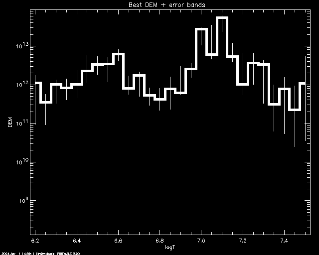
error bars from DEMERR (using SCHME 'ERRBAR'):
   PoA> mcmc_plot,logt,simdem,demerr,simprb,'ERRBAR'
        % LOADCT: Loading table B-W LINEAR

And to customize using PLOT keywords:
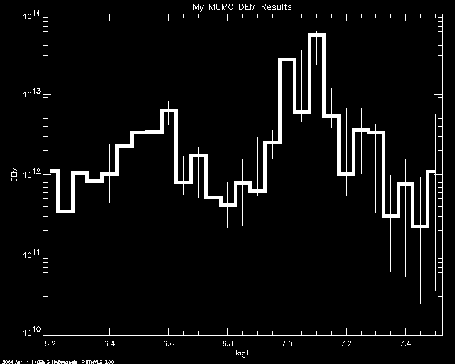
   PoA> mcmc_plot,logt,simdem,demerr,simprb,'ERRBAR',$
             yr = [1e10,1e14],title='My MCMC DEM Results'
        % LOADCT: Loading table B-W LINEAR

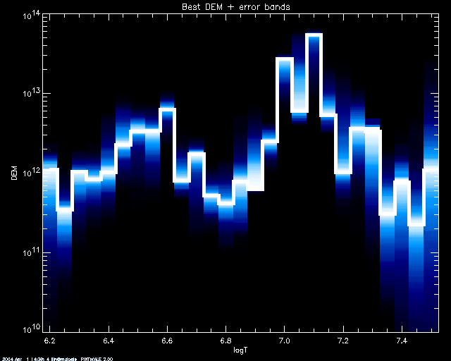
If one uses 'INDEX' , then each simulation value in each bin is
plotted and assigned a color corresponding to its index if counting from the
best simulation outwards. Colors are polyfilled between simulated
values. Here we set keyword COL_TABL =1 to choose a BLUE/WHITE color
table (see IDL documentation to find other color tables):
 PoA> mcmc_plot,logt,simdem,demerr,simprb,'INDEX',/yl, yr = [1e10,1e14],col_tabl=1
% LOADCT: Loading table BLUE/WHITE

By default, if using a SCHME other than 'ERRBAR', the best 50 %
simulated values (according to SIMPRB) are plotted. The CLEV
keyword may be used to toggle the percentage cutoff. The SLECT
keyword may be set to 1 to include all simulations or set to 3
to include simulations that fall within bounds set by DEMERR. (SLECT =
2 and CLEV = 50 are default values).
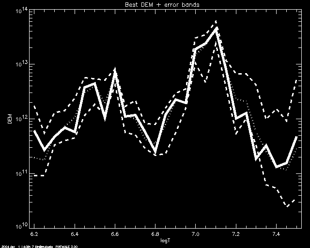
If one uses SCHME 'NICE', a median simulation value is calculated for
each bin. The median values will be plotted (dotted line) together with the DEM
simulation that best fits them (solid line). Uncertainty will be
displayed by plotting the minimum and maxim simulation values for each
bein (dashed lines). In this example we use SLECT = 3.
 PoA> mcmc_plot,logt,simdem,demerr,simprb,'NICE',/yl, yr= [1e10,1e14], slect=3
      % LOADCT: Loading table B-W LINEAR

- MCMC_ABUND uses MCMC_DEM
results to calculate fractional abundances relative to solar values
(Grevesse & Sauval 1998). Note that this function is to be used
for abundance-independent DEM-reconstructions i.e. those for which
flux ratios are used. The following parameters are required:
- -- simdem (MCMC_DEM keyword simdem)
- * an array of size (NT,NSIM+1) containing all
the sampled DEMS with the last column containing the
bestfit.
- * NT is the number of temperature bins on which the DEM
is defined and
- * NSIM is the number of simulations done to
sample the DEM parameter space.
- -- logt as described above, is the temperature grid of the reconstructed DEM
- -- wvl wavelengths [Ang]
- -- flx flux [ph/s] at each WVL ([ph/s/cm^2]
- -- fsigma errors for flx
- -- z atomic numbers of the elements
generating the lines at WVL.
- -- asig on output, contains the errors in the weighted mean abundances
- -- zout on output, atomic numbers corresponding to output abundances
The following keywords are accepted:
- -- elogt log_10(Temperature[K]) at which EMIS are defined if different from logt
- -- nosol if set, then output abundances will not be relative to solar
- -- olog if set, outputs abundances and asig will be logarithmic values.
- -- crctn_factor if set, correction factor is
applied to theoretical fluxes before calculation of abundnaces
To caclulate weighted mean abundances for the elements used in the DEM
reconstruction:
  PoA> restore, 'my_mcmc_run.save'
  PoA> wtd_mean_abund=mcmc_abund(simdem,logt,wvl,flx,fsigma,emis,z,asig,zout)
To calculate weighted mean abundances for all the elemnts contained in
the ID structure, first get the required feilds from the ID structure (see Prep the inputs for MCMC analysis above):
  PoA>	wavelengths = idstr.WVL
  PoA>  fluxes[iLAMBDA] = idstr.(iLAMBDA+1).FLUX
  PoA>  flux_errors[iLAMBDA] = idstr.(iLAMBDA+1).FLUXERR
  PoA>  emissivity[*,iLAMBDA] = idstr.(iLAMBDA+1).EMIS
  PoA>	Z = idstr.(iLAMBDA).Z
and then restore the MCMC_DEM save file and then call MCMC_ABUND with the
elogt keyword set to the temperture grid on which ID structure
emissivities are defined (usually PoA default !LOGT):
  PoA>  restore, 'my_mcmc_run.save'
  PoA>  wtd_mean_abund=mcmc_abund(simdem,logt,wavelengths,fluxes,flux_errors,$
        emissivity,Z,asig,zout,elogt=!LOGT)
To use these abundance values to say, calculate a synthetic spectrum
using PINTofALE
(e.g. see Simulating Chandra ACIS
spectra, Simulating Chandra
HETGS MEG spectra of density sensitive O VII lines and Simulating XMM EPIC-pn, EPIC-mos,
and RGS spectra), first use MCMC_ABUND with the NOSOL keyword set to get absolute
abundances (not relative to solar):
  PoA>  restore, 'my_mcmc_run.save'
  PoA>  wtd_mean_abund=mcmc_abund(simdem,logt,wavelengths,fluxes,flux_errors,$
         emissivity,Z,asig,zout,elogt=!LOGT,/nosol)
then get a PINTofALE style abundnace array using from GETABUND() (where z = INDEX-1):
PoA> abund=get_abund('grevesse & suval')
and replace the abundnaces for the elements for which you have
values::
PoA> abund(zout-1) = wtd_mean_abund
6. Example code
The following is an example code which follows the steps 1-4 of this
guide. The code assumes the follwing quantities are defined:
- -- a counts array countarr [cts/bin] defined on wavelength grid wvlarr [Ang]
- -- an effective area arrary effar [cm^2] on wvaelength grid awvlarr [Ang]
- -- an ascii list line_list as described above (Choose a set of lines from which to derive the DEM)
;      1. Choose spectral lines for analysis
  munge_list, 'line_list', idstr, rdlnlst

;      2. Fitting our chosen set of lines
  id_to_fitpar, idstr,pars,ties,thaw,pos=pos,wdt=wdt,lsfwdt=lsfwdt,$
               flx=flx,epithet = epithet

  fitstr = fitlines(wvlarr,countarr,pos=pos,wdt=wdt,$
           flx=flx,type=type,epithet=epithet,ties=ties,/dumb)
  save, fitstr,filename = 'fitstr.save'
; restore, 'fitstr.save',/v

;      3. Update the ID structure with fit information
  flxerr = (fitstr.ferrp+fitstr.ferrm)/2
  idstr  = updatid(idstr, fitstr.flx, fitstr.pos, flxerr=flxerr)

;      consolidate multiplets and prepare mproxy keyword
  idstr = squishem(idstr, mproxy=mproxy)

;      4. Preparing MCMC_DEM() input arrays
  nl = n_elements(idstr.wvl)
  flxs = fltarr(nl) & flxerrs = fltarr(nl) & wvls = fltarr(nl)
  emis = fltarr(n_elements(idstr.(1).logt),nl) & zs = fltarr(nl)

  for j = 1, nl do flxs(j-1) = idstr.(j).flux
  for j = 1, nl do flxerrs(j-1) = idstr.(j).fluxerr
  for j = 1, nl do wvls(j-1) = idstr.(j).wvl
  for j = 1, nl do emis(*,j-1) = idstr.(j).emis
  for j = 1, nl do zs(j-1) = idstr.(j).z

  newlogt = 6.2+findgen(17)*0.1

;      4.A Using line ratios
  ll = wvlarr(where(wvlar gt 2.4 and wvlar lt 3.4))
  wgrid = mid2bound(wvlarm)
  licospec,wgrid[ll],lspec,cspec,verbose=10,lstr=lstr,cstr=cstr,n_e=1e10,$
  lcthr = 0.05, constr=constr, lrf=lrf,type=type,LEMIS=LEMIS,CEMIS=CEMIS
  oo = where(lspec/cspec lt 0.05)
  tmp = countarr[ll]
;      filter at the 5 % level
  contflx = total(tmp(oo)) & contflxerr = 1+sqrt(0.75+contflx0)

;      get the continuum measurement and error
  conemis = constr.cont_int*(max(wgrid)-min(wgrid))
  conemis = rebinx(conemis, !logt, logt) & avgwvl0 = constr.midwvl

;      add the appropriate continuum quantities to our previously defined input arrays.
  fluxes      = [fluxes,contflx]
  fluxerr     = [flxerrs,contflxerr]
  wavelengths = [wavelengths,2.8]
  emissivity  = [emissivity,conemis]
  z           = [z,1]
  newemis = rebinx(emissivity,!logt, newlogt)

;      fold effective areas
  for j = 0, n_elements(fluxes) - 1 do $
      fluxes(j) = fluxes(j)/effar(where(hastogram(wavelengths(j),awvlarr) eq 1))
  for j = 0, n_elements(fluxes) - 1 do $
      fluxerr(j) = fluxes(j)/effar(where(hastogram(wavelengths(j),awvlarr) eq 1))

;      4.B Automatic deblending of lines

;      turn on automatic deblending of lines by setting MIXSSTR = 1
   MIXSSTR = 1

;      set MPROXY keyword (which may or may not be from SQUISHEM, here we asume it is)
   MPROXY = MPROXY

;      5. Now a call to MCMC_DEM()
  adem = mcmc_dem(wavelengths,fluxes,newemis,z=z,fsigma=flxerr,onlyrat=onlyrat,$
         mixsstr=mixsstr,logt=newlogt,mproxy=mproxy)


pintofale()head.cfa.harvard.edu (LL)
