Background Subtraction [EotW]
There is a lesson that statisticians, especially of the Bayesian persuasion, have been hammering into our skulls for ages: do not subtract background. Nevertheless, old habits die hard, and old codes die harder. Such is the case with X-ray aperture photometry.
When C counts are observed in a region of the image that overlaps a putative source, and B counts in an adjacent, non-overlapping region that is mostly devoid of the source, the question that is asked is, what is the intensity of a source that might exist in the source region, given that there is also background. Let us say that the source has intensity s, and the background has intensity b in the first region. Further let a fraction f of the source overlap that region, and a fraction g overlap the adjacent, “background” region. Then, if the area of the background region is r times larger, we can solve for s and b and even determine the errors:
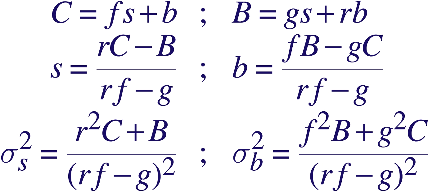
Note that the regions do not have to be circular, nor does the source have to be centered in it. As long as the PSF fractions f and g can be calculated, these formulae can be applied. In practice, f is large, typically around 0.9, and the background region is chosen as an annulus centered on the source region, with g~0.
It always comes as a shock to statisticians, but this is not ancient history. We still determine maximum likelihood estimates of source intensities by subtracting out an estimated background and propagate error by the method of moments. To be sure, astronomers are well aware that these formulae are valid only in the high counts regime ( s,C,B>>1, b>0 ) and when the source is well defined ( f~1, g~0 ), though of course it doesn’t stop them from pushing the envelope. This, in fact, is the basis of many standard X-ray source detection algorithms (e.g., celldetect).
Furthermore, it might come as a surprise to many astronomers, but this is also the rationale behind the widely-used wavelet-based source detection algorithm, wavdetect. The Mexican Hat wavelet used with it has a central positive bump, surrounded by a negative annular moat, which is a dead ringer for the source and background regions used here. The difference is that the source intensity is not deduced from the wavelet correlations and the signal-to-noise ratio ( s/sigmas ) is not used to determine source significance, but rather extensive simulations are used to calibrate it.
TomLoredo:
Vinay:
“…old habits die hard, and old codes die harder…
Ouch! I think you should copyright that!
05-22-2008, 11:45 pmhlee:
I’m still in doubt that why just b, not tb as rb in B=gs+rb or why b in S is same as in B. How sure b is homogeneous? Nonetheless, I’m sure that the given expressions work well and homogeneity is astrophysical correct.
06-08-2008, 8:12 pmvlk:
why just b, not tb as rb in B=gs+rb or why b in S is same as in B
say again?
06-08-2008, 9:37 pmhlee:
I wish I could address the problem with more sense, meaning modeling with statistically justifiable assumptions. The section 2.2 from this week’s arxiv:astro-ph paper describes Background Subtraction, which I couldn’t understand the procedure at the first glance ([astro-ph:0806.1575], more papers introducing background substarction are welcome). Is this the way how astronomers estimate b and s?
My question is, what is random and what is fixed? C and B are random variables following the Poisson distribution with given rates, that I don’t doubt. Yet, how come r and b are deterministic? How sure b is fixed and same for both equations in the first line? I bet checking S/N is to ensure gs is zero (or ignorable), though.
All I wish to get is any historic account that b is homogeneous and two b’s in the first line are the same (according to the account, r is a fixed value, independent of s, and I introduced t in tb to indicate that b is not necessarily homogeneous. The model would be written in different fashions).
06-10-2008, 11:54 pmvlk:
r is deterministic, because it is the ratio of areas (in units of [pix2 cm2 sec]) in which the counts C and B are collected. There may be systematic uncertainties here, but no statistical uncertainties.
b is not deterministic; it is the intensity of the background in the source area. Therefore, the area correction factor is unity, and there is no need to resort to extra variables t.
You are correct that an assumption is made that the background at an off-source location also describes the background under the source. But if you do not make this assumption, you will have 3 variables (s and b in the source region and say b’ in the background region) and 2 equations, so you will have to have another relation saying what b’ is as a function of b. As long as b’ is proportional to b, the proportionality constant can be subsumed into r and it will reduce without loss of generality to the same form as given above. If b’ is a non-linear function of b, well, you shouldn’t be using this formula then.
06-11-2008, 2:11 amhlee:
I have a rough idea to handle background in a general way, yet I do not know how to realize my idea with actual background and source data. A system of equations should not force the assumption of background homogeneity unless there’s a proof. I’m not opposing subtraction because to know the source flux, one should subtract background flux. Probably, I’ll get a well known obs id (well defined background region and source of nonignorable background) from CDA (Chandra Data Archive) and start playing with it to check feasibility of my idea! Even though it turns out into a vain, it could serve as an indirect proof of homogeneous background. But I’m afraid to tell you that getting used to a new tool and learning science behind it takes sometime.
06-24-2008, 4:52 pm