The AstroStat Slog

What is the maximum likelihood test in astronomy? Continue reading ‘my first AAS. II. maximum likelihood test’ »

High-resolution astronomical spectroscopy has invariably been carried out with gratings. Even with the advent of the new calorimeter detectors, which can measure the energy of incoming photons to an accuracy of as low as 1 eV, gratings are still the preferred setups for hi-res work below energies of 1 keV or so. But how do they work? Where are the sources of uncertainty, statistical or systematic?
Continue reading ‘Grating Dispersion [Equation of the Week]’ »

Despite no statistic related discussion, a paper comparing XSPEC and ISIS, spectral analysis open source applications might bring high energy astrophysicists’ interests this week. Continue reading ‘[ArXiv] 1st week, June 2008’ »

My first impression from the 212th AAS meeting is that it’s planned for preparing IYA 2009 and many talks are about current and future project reviews and strategies to reach public (People kept saying to me that winter meetings are more grand with expanded topics). I cannot say I understand everything (If someone says no astronomers understand everything, I’ll be relieved) but thanks to the theme of the meeting, I was intelligently entertained enough in many respects. The downside of this intellectual stimulus is growing doubts. One of those doubts was regression analysis in astronomy. Continue reading ‘my first AAS. I. Regression’ »

X-ray telescopes generally work by reflecting photons at grazing incidence. As you can imagine, even small imperfections in the mirror polishing will show up as huge roadbumps to the incoming photons, and the higher their energy, the easier it is for them to scatter off their prescribed path. So X-ray telescopes tend to have sharp peaks and fat tails compared to the much more well-behaved normal-incidence telescopes, whose PSFs (Point Spread Functions) can be better approximated as Gaussians.

X-ray telescopes usually also have gratings that can be inserted into the light path, so that photons of different energies get dispersed by different angles, and whose actual energies can then be inferred accurately by measuring how far away on the detector they ended up. The accuracy of the inference is usually limited by the width of the PSF. Thus, a major contributor to the LRF (Line Response Function) is the aforementioned scattering.

A correct accounting of the spread of photons of course requires a full-fledged response matrix (RMF), but as it turns out, the line profiles can be fairly well approximated with Beta profiles, which are simply Lorentzians modified by taking them to the power β –

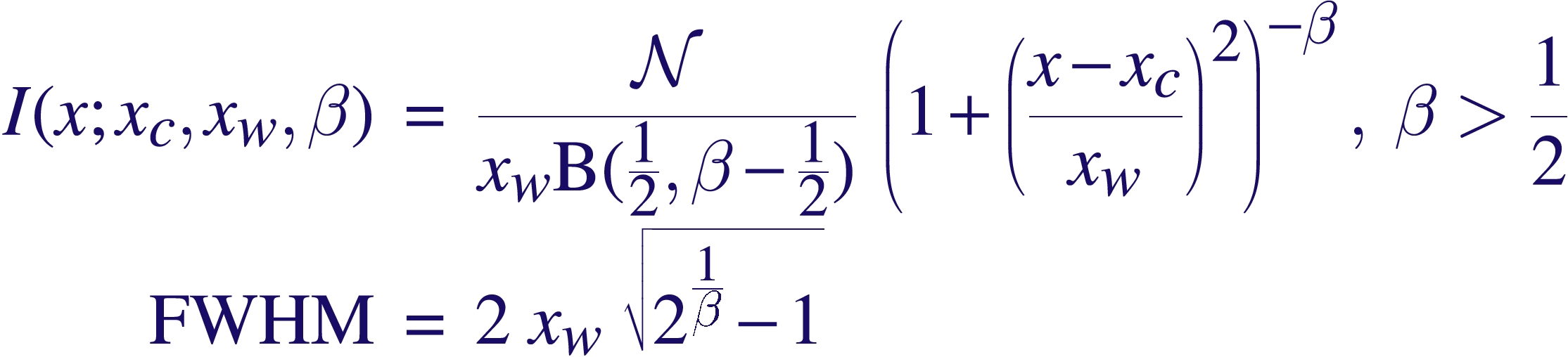
where B(1/2,β-1/2) is the Beta function, and N is a normalization constant defined such that integrating the Beta profile over the real line gives the area under the curve as N. The parameter β controls the sharpness of the function — the higher the β, the peakier it gets, and the more of it that gets pushed into the wings. Chandra LRFs are usually well-modeled with β~2.5, and XMM/RGS appears to require Lorentzians, β~1.

The form of the Lorentzian may also be familiar to people as the Cauchy Distribution, which you get for example when the ratio is taken of two quantities distributed as zero-centered Gaussians. Note that the mean and variance are undefined for that distribution.

It is somewhat surprising that astronomers haven’t cottoned on to Lowess curves yet. That’s probably a good thing because I think people already indulge in smoothing far too much for their own good, and Lowess makes for a very powerful hammer. But the fact that it is semi-parametric and is based on polynomial least-squares fitting does make it rather attractive.

And, of course, sometimes it is unavoidable, or so I told Brad W. When one has too many points for a regular polynomial fit, and they are too scattered for a spline, and too few to try a wavelet “denoising”, and no real theoretical expectation of any particular model function, and all one wants is “a smooth curve, damnit”, then Lowess is just the ticket.

Well, almost.

There is one major problem — how does one figure what the error bounds are on the “best-fit” Lowess curve? Clearly, each fit at each point can produce an estimate of the error, but simply collecting the separate errors is not the right thing to do because they would all be correlated. I know how to propagate Gaussian errors in boxcar smoothing a histogram, but this is a whole new level of complexity. Does anyone know if there is software that can calculate reliable error bands on the smooth curve? We will take any kind of error model — Gaussian, Poisson, even the (local) variances in the data themselves.