Last Updated: 2014jun15

IACHEC 2014

pyBLoCXS Demo

by Vinay Kashyap

Requirements | pyBLoCXS | arfmunge | AREF | Cal Uncertainty | References | changelog

This is a walkthrough of a demo on pyBLoCXS and calibration uncertainties conducted at IACHEC 2014 on May 12 by Vinay Kashyap (CXC/CHASC/CfA). The demo complements the talk on strategies to deal with systematic calibration errors from earlier in the day.

This document is split into multiple parts: the first gives details on the software and data that were used in the demo, and describes ways to get and install the necessary components; the second shows how to run the MCMC-based Bayesian spectral fitting algorithm (known as pyBLoCXS; van Dyk et al. 2001) in Sherpa; the third describes how to generate random sample curves of effective areas representative of known systematic errors using arfmunge; the fourth shows how to compress the resulting sample into a format that is flexible and portable, and which is currently implemented in Sherpa-pyBLoCXS; and the fifth shows how to carry out spectral analysis that includes calibration uncertainties.

Requirements

To follow through all the steps in this demo, the following are needed:

Data
We will use an ACIS-S aimpoint observation of Quasar Q1127-145 (ObsID 866) throughout. The source has >15000 counts, and should therefore be sensitive to calibration uncertainty.
The data files are in a gzipped tar file.
 
Sherpa
Sherpa is part of CIAO, which may be downloaded from cxc.harvard.edu/ciao/download
 
arfmunge
arfmunge is part of the MCcal package developed by Jeremy Drake (jdrake@cfa harvard edu) and Pete Ratzlaff (pratzlaff@cfa harvard edu). Please contact them directly to obtain a copy of the software.
arfmunge is written in perl, and requires the installation of modules PDL and Astro::FITS::CFITSIO from CPAN. First install cpanm with
cpan App::cpanminus
then run
cpanm PDL
cpanm Astro::FITS::CFITSIO
On Mac OS X, Astro::FITS::CFITSIO will be typically installed into ~/perl5/lib/perl5/darwin-thread-multi-2level/
We will assume that PDL is installed into
/home/username/perl5/lib/perl5/
and Astro::FITS::CFITSIO is installed into
/home/username/perl5/lib/perl5/darwin-thread-multi-2level/
and that MCCal itself is installed in the directory
$cwd/mccal-1.0/
 
R
R is a free statistics package, available from www.r-project.org.
See hea-www.harvard.edu/AstroStat/Tutorial2014/ for a tutorial by Eric Feigelson on using R.
The FITSio package is required in order to read in the FITS files. At the command line, do
install.packages("FITSio")
require("FITSio")
 
IDL or gnudatalanguage
The scripts for making AREF files are writtin in IDL (www.exelisinc.com/solutions/IDL/Pages/default.aspx). They are also compatible with gdl (gnudatalanguage.sourceforge.net).
In either case, they require that the IDLastro library (idlastro.gsfc.nasa.gov) be installed and its location be made available to the !PATH system variable.
 

pyBLoCXS in Sherpa

We will first demonstrate standard analysis. We will run a Sherpa fit, and then a Bayesian MCMC fit, and compare the results.

Unzip and untar the data:

unix> gunzip -c exampledata.tar.gz | tar xvf -
unix> ls obs866/
acis.arf
acis.asphist
acis.pi
acis.rmf
acis_bg.pi
Start up Sherpa and read the data in
unix> ciao
unix> sherpa
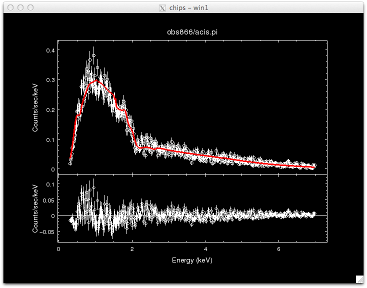
sherpa> load_data("obs866/acis.pi")
read ARF file obs866/acis.arf
read RMF file obs866/acis.rmf
read background file obs866/acis_bg.pi
Set up the fitting environment by fixing the energy range, setting up the source model, the fit statistic, and the fitting method.
sherpa> ignore(":0.3,7.0:") #0.3-7 keV
#(this is the step I forgot to do during the live demo at IACHEC)
sherpa> set_model(xsphabs.abs1*xspowerlaw.p1) #an absorbed power-law
sherpa> set_stat('cstat') #pyBLoCXS only works with cstat
sherpa> set_method('neldermead')
sherpa> fit()
Ignore warnings about background not being subtracted. With cstat, backgrounds may not be subtracted and must instead be modeled. We will ignore this complication for this demo.
sherpa> fit() #fit multiple times to ensure convergence
sherpa> covar()
covariance 1-sigma (68.2689%) bounds:
   Param            Best-Fit  Lower Bound  Upper Bound
   -----            --------  -----------  -----------
   abs1.nH          0.103681  -0.00569035   0.00569035
   p1.PhoIndex       1.24369   -0.0217466    0.0217466
   p1.norm       0.000581215 -1.26871e-05  1.26871e-05 
Display the fit, to make sure it looks OK.
sherpa> plot_fit_resid()
plot_fit_resid
Get the confidence bounds for later comparison (this will take some time).
sherpa> conf()
confidence 1-sigma (68.2689%) bounds:
   Param            Best-Fit  Lower Bound  Upper Bound
   -----            --------  -----------  -----------
   abs1.nH          0.103681  -0.00569035   0.00569035
   p1.PhoIndex       1.24369   -0.0217466    0.0217466
   p1.norm       0.000581215  -1.2588e-05  1.28854e-05
That both conf() and covar() produce similar values for the confidence bounds suggests that the likelihood surface is well-behaved and nearly parabolic near the best-fit.

Now, do a pyBLoCXS run. pyBLoCXS requires that a standard fit() and a covar() be run beforehand, so we can continue from where we stopped above. To run pyBLoCXS, we have to choose a sampler. There are four recognized currently in Sherpa, of which three are implemented.

sherpa> list_samplers()
         ['metropolismh', 'fullbayes', 'mh', 'pragbayes']
pragBayes is described in Lee et al. (2011). fullbayes (Xu et al. 2014) is not yet implemented. For standard analysis, we should choose MetropolisMH:
sherpa> set_sampler("MetropolisMH")

Then, call pyBLoCXS:
sherpa> stats, accept, params = get_draws(niter=500)

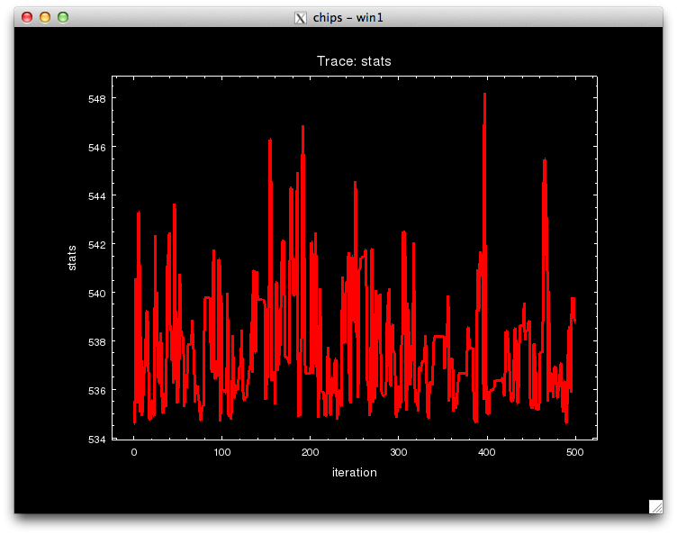
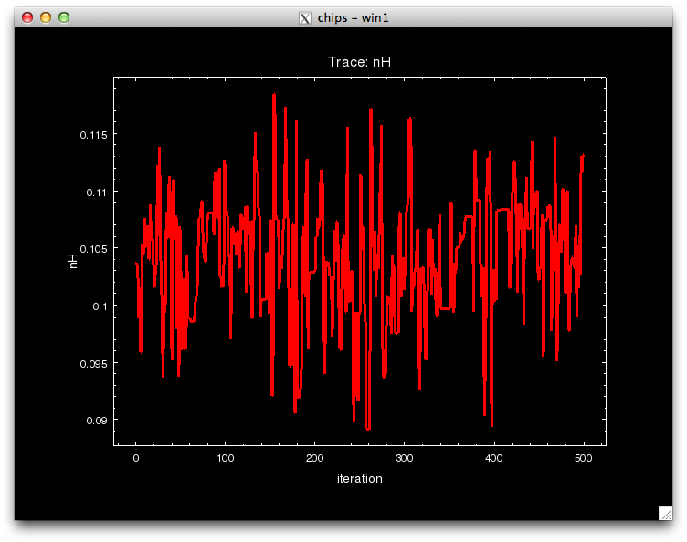
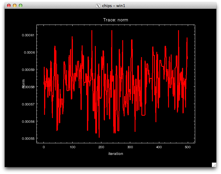
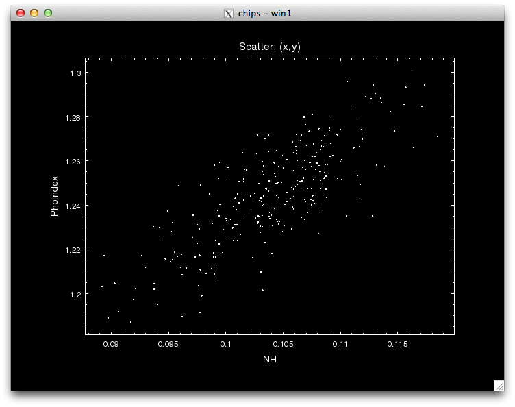
Notice that the call to pyBLoCXS is made through the function get_draws(), and it returns 3 outputs, the statistic value at each iteration, whether the draw was accepted or not, and the parameter values in the MCMC chain for each iteration, in that order.
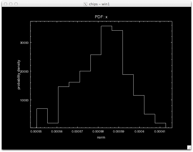
We can see see what the best-fit values are by finding the parameter values that correspond to the minimum statistic.
sherpa> bestfit = params[::,stats.argmin()].T sherpa> bestfit
array([  1.03680945e-01,   1.24369149e+00,   5.81215353e-04])
which are very close to the best-fit values. The error bars can be obtained as the standard deviations of the parameter traces.
sherpa> [params[i].std() for i in [0,1,2]]
[0.0054630064588717586, 0.021625075347852889, 1.2220452692220281e-05]
which are again very similar to the values derived with Sherpa. With all MCMC runs, it is a good idea to check that the traces look reasonable.
sherpa> plot_trace(stats,name="stats")
plot_trace_stats
sherpa> plot_trace(params[0],name="nH")
plot_trace_nH
sherpa> plot_trace(params[1],name="PhoIndex")
plot_trace_PhoIndex
sherpa> plot_trace(params[2],name="norm")
plot_trace_norm
We can also make scatter plots of one variable against another.
sherpa> plot_scatter(params[0],params[1],xlabel="nH",ylabel="PhoIndex")
plot_scatter_nH_PhoIndex
The posterior density functions look like this:
sherpa> plot_pdf(params[0],xlabel="nH")
plot_pdf_nH
sherpa> plot_pdf(params[1],xlabel="PhoIndex")
plot_pdf_PhoIndex
sherpa> plot_pdf(params[2],xlabel="norm")
plot_pdf_norm

pyBLoCXS takes the current values of its starting point, so different chains with different starting points can be run. Try setting, e.g.,

sherpa> abs1.nH=0.01 ; p1.PhoIndex=2.5
sherpa> stats_alt, accept_alt, params_alt = get_draws(niter=2000)
The first few hundred iterations must be discarded as the solutions burn-in. Parameter means and standard deviations computed from the later iterations are similar to previous calculations.

Making the Calibration Library: arfmunge

The calibration library is a set of calibration products generated as random samples based on an uncertainty model of the instrument. Jeremy Drake and Pete Ratzlaff have devised a scheme where various subsystem uncertainties are put together to generate a representative sample of possible calibration products (see Drake et al. 2006) This scheme is implemented in a package called MCCal, which generates ARFs and RMFs and fits a specified spectral model to each realization. Please contact them if you wish to try it out. Here, we will consider only Chandra/ACIS-S effective areas, and use the program arfgen (part of MCCal) to generate 500 realizations of the ARF for the Q1127-145 dataset considered above.

arfgen may be run in general as follows, assuming that (a) the perl modules PDL and FITSIOis installed in /home/username/perl5/lib/perl5/, (b) the FITSIO module

perl -I/home/username/perl5/lib/perl5/darwin-thread-multi-2level/ -I/home/username/perl5/lib/perl5/ ,/mccal-1.0/arfmunge obs866/acis.arf 866_sample.arf
An example shell script that generates 500 such random samples of ARFs is available here. The set of 500 ARFs generated thusly is available as a tar file here (it unpacks into a subdirectory named
store_arfs/866_0NN.arf

These ARFs can be read in to IDL

arf0=mrdfits('obs866/acis.arf',1,hdr) ;default ARF
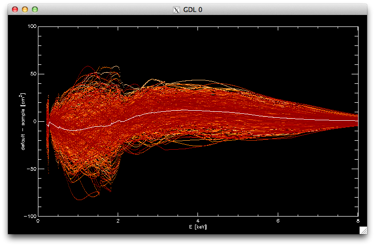
filarf=file_search('store_arfs/866_*.arf',count=narf) ;filenames of all randomly generated ARFs
arfs=fltarr(n_elements(arf0.SPECRESP),narf) ;array to hold all ARFs
for i=0L,narf-1L do begin & tmp=mrdfits(filarf[i],1,h) & arfs[*,i]=tmp.SPECRESP & endfor ;read in ARFs
and the difference between the default and the sample plotted
plot,[0],/nodata,xrange=[0.3,8],yrange=[-100,100],xtitle='E [keV]',ytitle='default - sample [cm!u2!n]' ;set up plot window
for i=0,narf-1 do oplot,arf0.ENERG_LO,arf0.SPECRESP-arfs[*,i],psym=3,color=((narf-i)/4)+100 ;plot the ARF library
oplot,arf0.ENERG_LO,arf0.SPECRESP-total(arfs,2)/narf ;plot the bias
arf_library_obs866
Similarly for the ratios, should you want to look at it that way
plot,[0],/nodata,xrange=[0.3,8],yrange=[0.8,1.2],/xs,/ys,xtitle='E [keV]',ytitle='default/sample [cm!u2!n]'
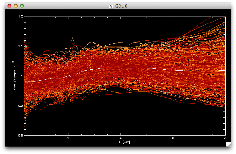
for i=0,narf-1 do oplot,arf0.ENERG_LO,arf0.SPECRESP/arfs[*,i],psym=3,color=((narf-i)/4)+100
oplot,arf0.ENERG_LO,arf0.SPECRESP/(total(arfs,2)/narf)
arf_by_library_obs866

Compressing the Calibration Library: AREF

The ARF calibration library computed above needs to be ingested into pyBLoCXS in a flexible manner. To do this, we have devised a file format called AREF (Ancillary Response Error Format; Kashyap et al.\ 2008) that is a superset of the OGOP ARF format, and is designed to allow for a large variety of uncertainties to be encoded.

These ARFs can also be consolidated and stored in a single file and used within pyBLoCXS. One of the AREF formats is a method called SIM1DADD. To construct it, use the IDL script samp2fits.pro, which produces the fits file 866_samp_aref.fits.

It is true that disk space is cheap, so there is the option of carrying around full sample libraries for each dataset. However, because such a strategy can quickly become unwieldy, and Principal Components compression provides other advantages (see Xu et al. 2014). So here we will show how to make an AREF file that utilizes the PCA1DADD method. We will first use an R script run_pca_on_arflib.r, which is a wrapper to the R program prcomp, to generate the Principal Components

R source("run_pac_on_arflib.r")
which produces the files
ls *_866.txt
avgarf_866.txt
pcomps_866.txt
sqlamb_866.txt
Then use an IDL script pca2aref.pro to generate the actual AREF file
idl
sqlambf='sqlamb_866.txt'
pcompf='pcomps_866.txt'
avgarff='avgarf_866.txt'
defarff='obs866/acis.arf'
areffil='866_pca_aref.fits'
vthresh=0.99
verbose=1
pca2aref, sqlambf, pcompf, avgarff, defarff, areffil, vthresh=vthresh, ncomp=ncomp, verbose=verbose

The SAMP AREF file has these extensions --

dmlist 866_samp_aref.fits blocks
     Block Name                          Type         Dimensions
--------------------------------------------------------------------------------
Block    1: PRIMARY                        Null        
Block    2: SPECRESP                       Table         6 cols x 1078     rows
Block    3: SIMCOMP                        Table         2 cols x 500      rows
and the PCA AREF file has these extensions --
dmlist 866_pca_aref.fits blocks
     Block Name                          Type         Dimensions
--------------------------------------------------------------------------------
Block    1: PRIMARY                        Null        
Block    2: SPECRESP                       Table         6 cols x 1078     rows
Block    3: PCACOMP                        Table         4 cols x 13       rows

Notice that 99% of the variability in the ARF library is accounted for with just 12 Principal Components (the 13th row in PCACOMP holds the residuals).

Accounting for Calibration Uncertainty

Here, we will demonstrate how to use the AREF files that contain calibration uncertainty information with pyBLoCXS. First, we have to set the sampler,

sherpa> set_sampler('pragbayes')
The sampler has the following fields:
sherpa> get_sampler()
{'defaultprior': True,
 'inv': False,
 'log': False,
 'nsubiters': 10,
 'originalscale': True,
 'p_M': 0.5,
 'priors': (),
 'priorshape': False,
 'scale': 1,
 'sigma_m': False,
 'simarf': None}
Notice the simarf field. That needs to be set to the AREF filename.
sherpa> set_sampler_opt('simarf', 'aref_866.fits')

Then, we run pyBLoCXS as above:
sherpa> stats_pB, accept_pB, params_pB = get_draws(niter=500)

This takes a substantial amount of time to run, because the code is carrying out fits at every iteration. A faster, optimized version has been developed, but has not been migrated to Sherpa yet. The new versioon also includes set_sampler('fullBayes'), and we plan to make it available in the near future via github.
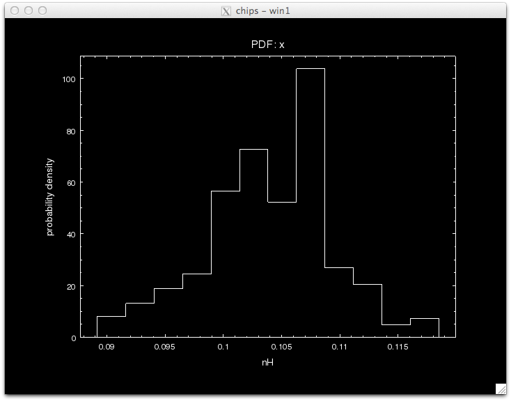
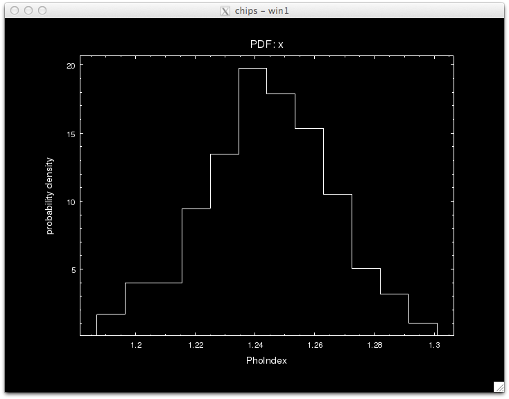
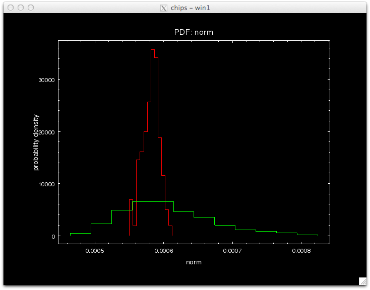
The standard and prag Bayes analyses may be compared using the posterior density distributions of the model parameters. (Note that the plots are made using a canned analysis; they will be updated using actual AREFs made here later.)
sherpa> plot_pdf(params[0],xlabel="nH",name="nH")
sherpa> plot_pdf(params_pB[0],overplot=True,clearwindow=False)
plot_pdf_nH_std_pB
sherpa> plot_pdf(params[1],xlabel="PhoIndex",name="PhoIndex")
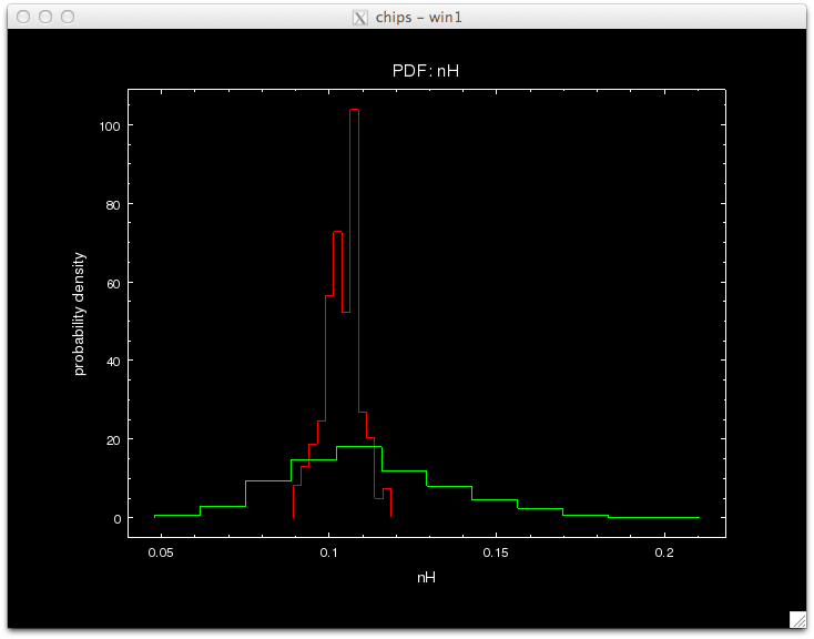
sherpa> plot_pdf(params_pB[1],overplot=True,clearwindow=False)
plot_pdf_PhoIndex_std_pB
sherpa> plot_pdf(params[2],xlabel="norm",name="norm")
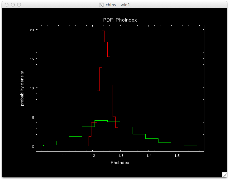
sherpa> plot_pdf(params_pB[2],overplot=True,clearwindow=False)
plot_pdf_norm_std_pB

References

Drake et al. 2006, SPIE 62701I
2006SPIE.6270E..49D
Kashyap et al. 2008, SPIE 7016, 21
2008SPIE.7016E..21K
@CDA [.pdf]
Lee et al. 2011, ApJ, 731, 126
2011ApJ...731..126L
OGIP ARF standard
heasarc.gsfc.nasa.gov/docs/heasarc/caldb/docs/memos/cal_gen_92_002/cal_gen_92_002.html
van Dyk et al. 2001, ApJ, 548, 224
2001ApJ...548..224V
Xu et al. 2014, ApJ, 794, 97
article [.pdf]

changelog

2014-may-27: set up page.
2014-jun-15: public version
2015-feb-18: updated link to Xu et al.


IACHEC 2014
pyBLoCXS Demo
by Vinay Kashyap
May 12 2014
Requirements
pyBLoCXS in Sherpa
Cal Library: arfmunge
Cal Library: AREF
Cal Errors and Sherpa
References
changelog


Vinay Kashyap <vkashyap @ cfa . harvard . edu>