Basic Fitting

Simple 1-D model fitting

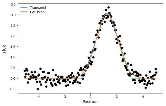
In this section, we look at a simple example of fitting a Gaussian to a simulated dataset. We use the Gaussian1D and Trapezoid1D models and the LevMarLSQFitter fitter to fit the data:

import numpy as np
import matplotlib.pyplot as plt
from astropy.modeling import models, fitting

# Generate fake data
np.random.seed(0)
x = np.linspace(-5., 5., 200)
y = 3 * np.exp(-0.5 * (x - 1.3)**2 / 0.8**2)
y += np.random.normal(0., 0.2, x.shape)

# Fit the data using a box model.
# Bounds are not really needed but included here to demonstrate usage.
t_init = models.Trapezoid1D(amplitude=1., x_0=0., width=1., slope=0.5,
                            bounds={"x_0": (-5., 5.)})
fit_t = fitting.LevMarLSQFitter()
t = fit_t(t_init, x, y)

# Fit the data using a Gaussian
g_init = models.Gaussian1D(amplitude=1., mean=0, stddev=1.)
fit_g = fitting.LevMarLSQFitter()
g = fit_g(g_init, x, y)

# Plot the data with the best-fit model
plt.figure(figsize=(8,5))
plt.plot(x, y, 'ko')
plt.plot(x, t(x), label='Trapezoid')
plt.plot(x, g(x), label='Gaussian')
plt.xlabel('Position')
plt.ylabel('Flux')
plt.legend(loc=2)

(png, svg, pdf)

As shown above, once instantiated, the fitter class can be used as a function that takes the initial model (t_init or g_init) and the data values (x and y), and returns a fitted model (t or g).

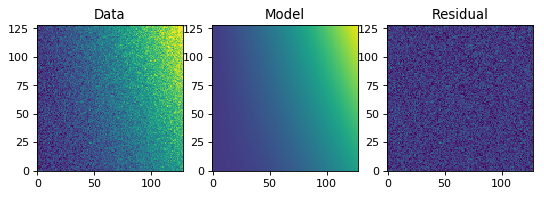
Simple 2-D model fitting

Similarly to the 1-D example, we can create a simulated 2-D data dataset, and fit a polynomial model to it. This could be used for example to fit the background in an image.

import warnings
import numpy as np
import matplotlib.pyplot as plt
from astropy.modeling import models, fitting

# Generate fake data
np.random.seed(0)
y, x = np.mgrid[:128, :128]
z = 2. * x ** 2 - 0.5 * x ** 2 + 1.5 * x * y - 1.
z += np.random.normal(0., 0.1, z.shape) * 50000.

# Fit the data using astropy.modeling
p_init = models.Polynomial2D(degree=2)
fit_p = fitting.LevMarLSQFitter()

with warnings.catch_warnings():
    # Ignore model linearity warning from the fitter
    warnings.simplefilter('ignore')
    p = fit_p(p_init, x, y, z)

# Plot the data with the best-fit model
plt.figure(figsize=(8, 2.5))
plt.subplot(1, 3, 1)
plt.imshow(z, origin='lower', interpolation='nearest', vmin=-1e4, vmax=5e4)
plt.title("Data")
plt.subplot(1, 3, 2)
plt.imshow(p(x, y), origin='lower', interpolation='nearest', vmin=-1e4,
           vmax=5e4)
plt.title("Model")
plt.subplot(1, 3, 3)
plt.imshow(z - p(x, y), origin='lower', interpolation='nearest', vmin=-1e4,
           vmax=5e4)
plt.title("Residual")

(png, svg, pdf)

The fitting framework includes many useful features that are not demonstrated here, such as weighting of datapoints, fixing or linking parameters, and placing lower or upper limits on parameters. For more information on these, take a look at the Fitting Models to Data documentation.