Welcome to pyBLoCXS documentation!
pyBLoCXS is a sophisticated Markov chain Monte Carlo (MCMC) based algorithm designed to carry out Bayesian Low-Count X-ray Spectral (BLoCXS) analysis in the Sherpa environment. The code is a Python extension to Sherpa that explores parameter space at a suspected minimum using a predefined Sherpa model to high-energy X-ray spectral data. pyBLoCXS includes a flexible definition of priors and allows for variations in the calibration information. It can be used to compute posterior predictive p-values for the likelihood ratio test (see Protassov et al., 2002, ApJ, 571, 545). Future versions will allow for the incorporation of calibration uncertainty (Lee et al., 2011, ApJ, 731, 126).
MCMC is a complex computational technique that requires some sophistication on the part of its users to ensure that it both converges and explores the posterior distribution properly. The pyBLoCXS code has been tested with a number of simple single-component spectral models. It should be used with great care in more complex settings. Readers interested in Bayesian low-count spectral analysis should consult van Dyk et al. (2001, ApJ, 548, 224). pyBLoCXS is based on the methods in van Dyk et al. (2001) but employs a different MCMC sampler than is described in that article. In particular, pyBLoCXS has two sampling modules. The first uses a Metropolis-Hastings jumping rule that is a multivariate t-distribution with user specified degrees of freedom centered on the best spectral fit and with multivariate scale determined by the Sherpa function, covar(), applied to the best fit. The second module mixes this Metropolis Hastings jumping rule with a Metropolis jumping rule centered at the current draw, also sampling according to a t-distribution with user specified degrees of freedom and multivariate scale determined by a user specified scalar multiple of covar() applied to the best fit.
A general description of the MCMC techniques we employ along with their convergence diagnostics can be found in Appendices A.2 - A 4 of van Dyk et al. (2001) and in more detail in Chapter 11 of Gelman, Carlin, Stern, and Rubin (Bayesian Data Analysis, 2nd Edition, 2004, Chapman & Hall/CRC).
Download
September 15, 2010 pyblocxs-0.0.3.tar.gz
Dependencies
pyBLoCXS requires
Sherpa 4.2.1 or later [sherpa]: A 1D/2D modeling and fitting application written as a set of Python modules.
| [sherpa] | http://cxc.harvard.edu/contrib/sherpa |
Documentation
The code is developed as Chandra contributed software.
Setup Instructions
To run it within CIAO/Sherpa, cd to .../pyblocxs-0.0.3, start Sherpa, and type import pyblocxs.
Or
To run it directly in Python, cd to .../pyblocxs-0.0.3, and and then type:
python setup.py install --prefix=<dest dir>
setenv PYTHONPATH ${PYTHONPATH}:<dest dir>/lib/python2.6/site-packages
python
and then from the Python prompt:
from pyblocxs import *
Alternatively, the tarball can be downloaded and unpacked to a location /path/to/pyblocxs. Python scripts should include the following lines before calling pyBLoCXS functions:
import sys
sys.path.append('/path/to/pyblocxs/pyblocxs-0.0.3')
import pyblocxs
Usage
The primary way to run pyBLoCXS within Sherpa is to call the function pyblocxs.get_draws()
First read in the spectrum:
load_pha("pha.fits")
and define the model:
set_model(xsphabs.abs1*powlaw1d.p1)
and carry out a regular fit to define the covariance matrix:
set_stat("cash")
fit()
covar()
then invoke pyBLoCXS with MetropolisMH as follows:
import pyblocxs
pyblocxs.set_sampler("MetropolisMH")
stats, accept, params = pyblocxs.get_draws(niter=1e4)
to change to MH:
pyblocxs.set_sampler("MH")
stats, accept, params = pyblocxs.get_draws(niter=1e4)
Listing of Control Parameters
Metropolis-Hastings Jumping Rule
- defaultprior – Boolean to indicate that all parameters have the default flat prior.
- inv – Boolean or array of booleans indicating which parameters are on the inverse scale.
- log – Boolean or array of booleans indicating which parameters are on the logarithm scale (natural log).
- originalscale – Array of booleans indicating which parameters are on the original scale.
- priorshape – Array of booleans indicating which parameters have associated user-defined prior functions.
- scale – A scalar multiple of the output of covar() used in the scale of the t-distribution.
Mixture of Metropolis and Metropolis-Hastings Jumping Rules
- defaultprior – Boolean to indicate that all parameters have the default flat prior.
- inv – Boolean or array of booleans indicating which parameters are on the inverse scale.
- log – Boolean or array of booleans indicating which parameters are on the logarithm scale (natural log).
- originalscale – Array of booleans indicating which parameters are on the original scale.
- p_M – The proportion of jumps generated by the Metropolis jumping rule.
- priorshape – Array of booleans indicating which parameters have associated user-defined prior functions.
- scale – A scalar multiple of the output of covar() used in the scale of the t-distribution
Passing Parameters
Users can set control parameters at a high level using set_sampler_opt():
set_sampler("MH")
set_sampler_opt("scale", 0.5)

set_sampler("MetropolisMH")
set_sampler_opt("p_M", 0.33)
Displaying the Results
The best-fit parameter values can be extracted as either:
bestfit = params[::,stats.argmin()].T
or:
npars = len(get_model().thawedpars)
bestfit = [params[ii][stats.argmin()] for ii in range(npars)]
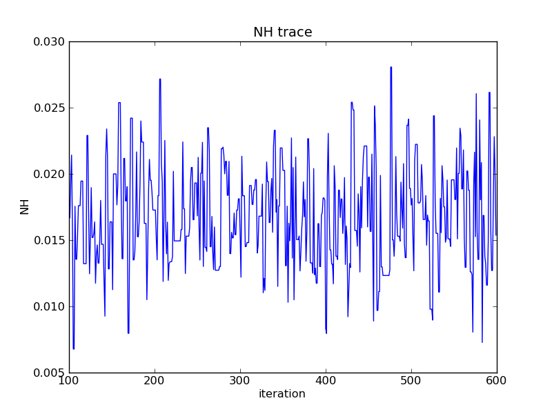
A simple trace of the parameter draws with burn-in:
import matplotlib.pyplot as pyplot
NHarr = params[0][nburn:niter]
pyplot.plot(range(nburn,niter), NHarr)
pyplot.xlabel("iteration")
pyplot.ylabel("NH")
pyplot.title("NH trace")
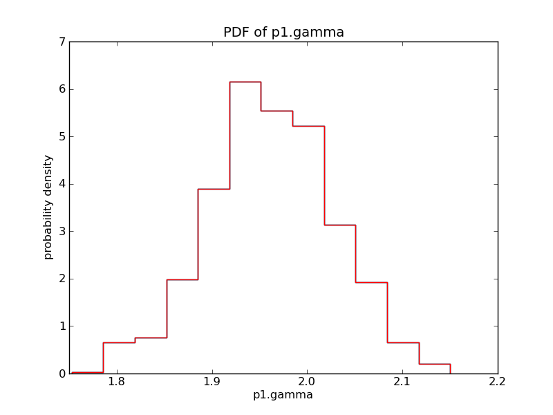
Histograms of the parameter draws can be made using matplotlib, as follows:
import matplotlib.pyplot as pyplot
pdf,bins,patches = pyplot.hist(params[0], bins=N, normed=True, histtype='step')
Or, using the plotting backend in Sherpa with:
pyblocxs.plot_pdf(params[0], name="abs1.nH", bins=N)
The draws can be filtered using NumPy array slicing:
nh_draws = params[0]

# only use (100,600], meaning 101st to 600th.
nh_draws_filtered = nh_draws[100:600]

pyblocxs.plot_pdf(nh_draws_filtered, "abs1.nh")
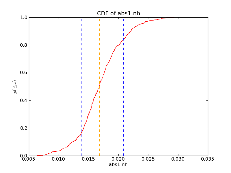
Quantiles of the parameter draws can be plotted using matplotlib:
import matplotlib
import matplotlib.pyplot as pyplot
import numpy

name = "abs1.nh"
x = numpy.sort(params[0])
median, lval, hval = pyblocxs.get_error_estimates(x, True)
y = (numpy.arange(x.size) + 1) * 1.0 / x.size

pyplot.plot(x, y, color='red')
pyplot.axvline(median, linestyle='--', color='orange')
pyplot.axvline(lval, linestyle='--', color='blue')
pyplot.axvline(hval, linestyle='--', color='blue')
pyplot.xlabel(name)
pyplot.ylabel(r"$p(\leq x)$")  # p(<= x)
pyplot.title("CDF of %s" % name)
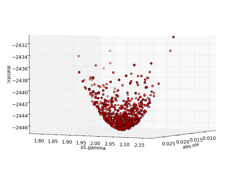
3D scatter plots of parameter space can be made using matplotlib:
from mpl_toolkits.mplot3d import Axes3D
import matplotlib.pyplot as pyplot

fig = pyplot.figure()
ax = Axes3D(fig)
ax.scatter(params[0], params[1], stats, c="red")
ax.set_xlabel("abs1.nh")
ax.set_ylabel("p1.gamma")
ax.set_zlabel("statistic")
pyplot.draw()
Priors
By default, pyBLoCXS uses a flat prior defined between the hardcoded parameter minima and maxima. But more informative priors can also be defined using the set_prior() function. if a model has been defined as, say, xsapec.therm, a Gaussian prior can be imposed on the temperature parameter by defining:
normgauss1d.g1
g1.pos=2.5; g1.fwhm=0.5
set_prior(therm.kT,g1)
set_sampler_opt('defaultprior', False)
set_sampler_opt('priorshape', [True, False, False])
set_sampler_opt('originalscale', [True, True, True])
Arbitrary functions can be defined by the user for use as priors:
def lognorm(x, sigma=0.5, norm=1.0, x0=20.):
   xl=numpy.log10(x)+22.
   return (norm/numpy.sqrt(2*numpy.pi)/sigma)*numpy.exp(-0.5*(xl-x0)*(xl-x0)/sigma/sigma)
and which can be invoked as, e.g.:
set_prior(abs1.NH,lognorm)
set_sampler_opt('defaultprior', False)
set_sampler_opt('priorshape', [True, False, False])
set_sampler_opt('originalscale', [True, True, True])
Transformations
Because the jumping rules employed by pyBLoCXS are all based on symmetric bell-shaped t-distributions, the MCMC code will be far more efficient if the posterior distribution is roughly bell-shaped. When this is not the case under the canonical parameterization of the fitted model, it can still often be true under some transformation of the canonical parameterization. For example we may replace a strictly positive parameter that has a right skewed posterior distribution with the log of that same parameter. pyBLoCXS allows for uni-variate transformations of any or all of the model parameters onto the log and inverse scales.
Given a set of five thawed parameter values where the first and third parameter are to be on the log scale:
set_sampler_opt('log', [True, False, True, False, False])
Similarly, if the last parameter is to be inverted:
set_sampler_opt('inv', [False, False, False, False, True])
API User Interface functions
- class pyblocxs.mh.MH(fit, sigma, mu, dof)[source]
The Metropolis Hastings Sampler
- accept(current, current_stat, proposal, proposal_stat, **kwargs)[source]
Should the proposal be accepted (using the Cash statistic and the t distribution)?
- class pyblocxs.mh.MetropolisMH(fit, sigma, mu, dof)[source]
The Metropolis Metropolis-Hastings Sampler
- accept(current, current_stat, proposal, proposal_stat, **kwargs)[source]
Should the proposal be accepted (using the Cash statistic and the t distribution)?
High-Level User Interface functions
- list_priors()
List the dictionary of currently set prior functions for the set of thawed Sherpa model parameters
- get_prior(par)
Return the prior function set for the input Sherpa parameter par:
func = get_prior(abs1.nh)
- set_prior(par, prior)
Set a prior function prior for the the input Sherpa parameter par. The function signature for prior is of the form lambda x.
- set_sampler(sampler)
Set a sampler type sampler as the default sampler for use with pyblocxs. sampler should be of type str. Native samplers available include “MH” and “MetropolisMH”. The default sampler is “MetropolisMH”. For example:
set_sampler("MetropolisMH")
- get_sampler_name()
Return the name of the currently set sampler type. For example:
print get_sampler_name()
"MH"
- get_sampler()
Return the current sampler’s Python dictionary of configuration options. For example:
print get_sampler()
"{'priorshape': False, 'scale': 1, 'log': False, 'defaultprior': True,
'inv': False, 'sigma_m': False, 'priors': (), 'originalscale': True,
'verbose': False}"
- set_sampler_opt(opt, value)
Set a configuration option for the current sampler type. A collection of configuration options is found by calling get_sampler() and examining the Python dictionary. For example:
# Set all parameters to log scale
set_sampler_opt('log', True)

# Set only the first parameter to log scale
set_sampler_opt('log', [True, False, False])
- get_sampler_opt(opt)
Get a configuration option for the current sampler type. A collection of configuration options is found by calling get_sampler() and examining the Python dictionary. For example:
get_sampler_opt('log')
False
- get_draws(id=None, otherids=(), niter=1e3)
Run pyblocxs using current sampler and current sampler configuration options for niter number of iterations. The results are returned as a 3-tuple of Numpy ndarrays. The tuple specifys an array of statistic values, an array acceptance booleans, and a 2-D array of associated parameter values. The arguments id and otherids are used to access the Sherpa fit object to be used in the run by Sherpa data id. Note, before running get_draws a Sherpa fit must be complete and the covariance matrix should be calculated at the resultant fit minimum. For example:
stats, accept, params = get_draws(1, niter=1e4)
- get_error_estimates(x, sorted=False)
Compute the quantiles and return the median, -1 sigma value, and +1 sigma value for the array x. The sorted argument indicates whether x has been sorted. For example:
median, low_val, hi_val = get_error_estimates(x, sorted=True)
- plot_pdf(x, name='x', bins=12, overplot=False)
Compute a histogram and plot the probability density function of x. For example:
import numpy as np
mu, sigma = 100, 15
x = mu + sigma*np.random.randn(10000)
plot_pdf(x, bins=50)