Examples
Evaluating a one-dimensional model directly
In the following example a one-dimensional gaussian is evaluated on a grid of 5 points. The first approch calls the model directly, which uses the parameter values as defined in the model itself:
>>> from sherpa.models.basic import Gauss1D
>>> gmdl = Gauss1D()
>>> gmdl.fwhm = 100
>>> gmdl.pos = 5050
>>> gmdl.ampl = 50
>>> x = [4800, 4900, 5000, 5100, 5200]
>>> y1 = gmdl(x)
The second uses the calc() method, where the parameter values are
included in the call. The order matches that of the parameters in
the model, which can be found from the
pars attribute of the model:
>>> [p.name for p in gmdl.pars]
['fwhm', 'pos', 'ampl']
>>> y2 = gmdl.calc([100, 5050, 100], x)
>>> y2 / y1
array([ 2.,  2.,  2.,  2.,  2.])
Since the amplitude is twice that used to create y1 the ratio is
2 for each bin.
Evaluating a 2D model to match a Data2D object
In the following example the model is evaluated on a grid
specified by a dataset, in this case a set of two-dimensional
points stored in a Data2D object.
First the data is set up (there are only four points
in the dataset).
>>> from sherpa.data import Data2D
>>> x0 = [1.0, 1.9, 2.4, 1.2]
>>> x1 = [-5.0, -7.0, 2.3, 1.2]
>>> y = [12.1, 3.4, 4.8, 5.2]
>>> twod = Data2D('data', x0, x1, y)
For demonstration purposes, the Box2D
model is used, which represents a rectangle (any points within the
xlow
to
xhi
and
ylow
to
yhi
limits are set to the
ampl
value, those outside are zero).
>>> from sherpa.models.basic import Box2D
>>> mdl = Box2D('mdl')
>>> mdl.xlow = 1.5
>>> mdl.xhi = 2.5
>>> mdl.ylow = -9.0
>>> mdl.yhi = 5.0
>>> mdl.ampl = 10.0
The coverage have been set so that some of the points are within the “box”, and so are set to the amplitude value when the model is evaluated.
>>> twod.eval_model(mdl)
array([  0.,  10.,   10.,   0.])
The eval_model() method evaluates
the model on the grid defined by the data set, so it is the same
as calling the model directly with these values:
>>> twod.eval_model(mdl) == mdl(x0, x1)
array([ True,  True,  True,  True], dtype=bool)
The eval_model_to_fit() method
will apply any filter associated with the data before
evaluating the model. At this time there is no filter
so it returns the same as above.
>>> twod.eval_model_to_fit(mdl)
array([  0.,  10.,   10.,   0.])
Adding a simple spatial filter - that excludes one of
the points within the box - with
ignore() now results
in a difference in the outputs of
eval_model()
and
eval_model_to_fit(),
as shown below. The call to
get_indep()
is used to show the grid used by
eval_model_to_fit().
>>> twod.ignore(x0lo=2, x0hi=3, x1l0=0, x1hi=10)
>>> twod.eval_model(mdl)
array([  0.,  10.,   10.,   0.])
>>> twod.get_indep(filter=True)
(array([ 1. ,  1.9,  1.2]), array([-5. , -7. ,  1.2]))
>>> twod.eval_model_to_fit(mdl)
array([  0.,  10.,   0.])
Evaluating a model using a DataPHA object
Note
Not convinced model evaluation is correct here; do I need to add the instrument model in or not? I am pretty sure that, as written, it does not include the response information. So, could compare model evaluation without and with the instrument model.
This example is similar to the
two-dimensional case above,
in that it again shows the differences between the
eval_model()
and
eval_model_to_fit()
methods. The added complication in this
case is that the response information provided with a PHA file
is used to convert between the “native” axis of the
PHA file (channels) and that of the model (energy or
wavelength). This conversion is handled automatically
by the two methods (the
following example
shows how this can be done manually).
To start with, the data is loaded from a file, which also loads in the associated ARF and RMF files):
>>> from sherpa.astro.io import read_pha
>>> pha = read_pha('3c273.pi')
WARNING: systematic errors were not found in file '3c273.pi'
statistical errors were found in file '3c273.pi'
but not used; to use them, re-read with use_errors=True
read ARF file 3c273.arf
read RMF file 3c273.rmf
>>> pha
<DataPHA data set instance '3c273.pi'>
>>> pha.get_arf()
<DataARF data set instance '3c273.arf'>
>>> pha.get_rmf()
<DataRMF data set instance '3c273.rmf'>
The returned object - here pha - is an instance of the
sherpa.astro.data.DataPHA class - which has a number
of attributes and methods specialized to handling PHA data.
This particular file has grouping information in it, that it it contains
GROUPING and QUALITY columns, so Sherpa
applies them: that is, the number of bins over which the data is
analysed is smaller than the number of channels in the file because
each bin can consist of multiple channels. For this file,
there are 46 bins after grouping (the filter argument to the
get_dep() call applies both
filtering and grouping steps, but so far no filter has been applied):
>>> pha.channel.size
1024
>>> pha.get_dep().size
1024
>>> pha.grouped
True
>>> pha.get_dep(filter=True).size
46
A filter - in this case to restrict to only bins that cover the
energy range 0.5 to 7.0 keV - is applied with the
notice() call, which
removes 4 bins:
>>> pha.set_analysis('energy')
>>> pha.notice(0.5, 7.0)
>>> pha.get_dep(filter=True).size
42
A power-law model (PowLaw1D) is
created and evaluated by the data object:
>>> from sherpa.models.basic import PowLaw1D
>>> mdl = PowLaw1D()
>>> y1 = pha.eval_model(mdl)
>>> y2 = pha.eval_model_to_fit(mdl)
>>> y1.size
1024
>>> y2.size
42
The eval_model() call
evaluates the model over the full dataset and does not
apply any grouping, so it returns a vector with 1024 elements.
In contrast, eval_model_to_fit()
applies both filtering and grouping, and returns a vector that
matches the data (i.e. it has 42 elements).
The filtering and grouping information is dynamic, in that it
can be changed without having to re-load the data set. The
ungroup() call removes
the grouping, but leaves the 0.5 to 7.0 keV energy filter:
>>> pha.ungroup()
>>> y3 = pha.eval_model_to_fit(mdl)
>>> y3.size
644
Note
TODO: add in a way to get the X axis after grouping, if we have it; maybe the apply_grouping call of the data object? Or the to_fit option? Also to_plot.
Evaluating a model using PHA responses
Note
Should this just use Response1D directly?
The sherpa.astro.data.DataPHA class handles the
response information automatically, but it is possible to
directly apply the response information to a model using
the sherpa.astro.instrument module. In the following
example the
RSPModelNoPHA
and
RSPModelPHA
classes are used to wrap a power-law model
(PowLaw1D)
so that the
instrument responses - the ARF and RMF -
are included in the model evaluation.
>>> from sherpa.astro.io import read_arf, read_rmf
>>> arf = read_arf('3c273.arf')
>>> rmf = read_rmf('3c273.rmf')
>>> rmf.detchans
1024
The number of channels in the RMF - that is, the number of bins over which the RMF is defined - is 1024.
>>> from sherpa.models.basic import PowLaw1D
>>> mdl = PowLaw1D()
The RSPModelNoPHA class
models the inclusion of both the ARF and RMF:
>>> from sherpa.astro.instrument import RSPModelNoPHA
>>> inst = RSPModelNoPHA(arf, rmf, mdl)
>>> inst
<RSPModelNoPHA model instance 'apply_rmf(apply_arf(powlaw1d))'>
>>> print(inst)
apply_rmf(apply_arf(powlaw1d))
   Param        Type          Value          Min          Max      Units
   -----        ----          -----          ---          ---      -----
   powlaw1d.gamma thawed            1          -10           10
   powlaw1d.ref frozen            1 -3.40282e+38  3.40282e+38
   powlaw1d.ampl thawed            1            0  3.40282e+38
The output above suggests that the inst variable behaves as a
normal Shepra model, which it does:
>>> from sherpa.models.model import ArithmeticModel
>>> isinstance(inst, ArithmeticModel)
True
>>> inst.pars
(<Parameter 'gamma' of model 'powlaw1d'>,
 <Parameter 'ref' of model 'powlaw1d'>,
 <Parameter 'ampl' of model 'powlaw1d'>)
The model can therefore be evaluated, for instance by calling it with a grid (as used in the first example above), except that the input grid is ignored and the “native” grid of the response information is used: in this case the 1024 channels of the RMF.
>>> inst([0.1, 0.2, 0.3])
array([ 0.,  0.,  0., ...,  0.,  0.,  0.])
>>> inst([0.1, 0.2, 0.3])
array([ 0.,  0.,  0., ...,  0.,  0.,  0.])
>>> inst([0.1, 0.2, 0.3]).size
1024
>>> inst([10, 20]) == inst([])
array([ True,  True,  True, ...,  True,  True,  True], dtype=bool)
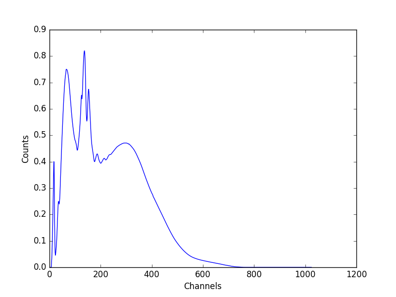
The output of this call represents the number of counts expected in each bin.
>>> ydet = inst([])
>>> chans = np.arange(rmf.offset, rmf.offset + rmf.detchans)
>>> plt.plot(x, ydet)
>>> plt.xlabel('Channels')
>>> plt.ylabel('Counts')
The data in the EBOUNDS extension of the RMF - which provides
an approximate mapping from channel to energy for visualization
purposes only - is available as the
e_min
and
e_max
attributes of the
DataRMF object returned by
read_rmf(). The plot can therefore
be re-created with energy units for the abscissa:
>>> print(rmf)
name     = sherpa-test-data/sherpatest/3c273.rmf
detchans = 1024
energ_lo = Float64[1090]
energ_hi = Float64[1090]
n_grp    = UInt64[1090]
f_chan   = UInt64[2002]
n_chan   = UInt64[2002]
matrix   = Float64[61834]
offset   = 1
e_min    = Float64[1024]
e_max    = Float64[1024]
>>> emid = (rmf.e_min + rmf.e_max) / 2
>>> plt.plot(emid, ydet)
>>> plt.xlabel('Energy (keV)')
>>> plt.ylabel('Counts')

The
RSPModelPHA
class adds in a
DataPHA object, which lets the
evaluation grid be determined by any filter applied to the
data object. In the following, the
read_pha() call reads in a PHA
file, along with its associated ARF and RMF (because the
ANCRFILE and RESPFILE keywords are set in the
header of the PHA file), which means that there is no need
to call
read_arf()
and
read_rmf()
to creating the RSPModelPHA instance.
>>> from sherpa.astro.io import read_pha
>>> from sherpa.astro.instrument import RSPModelPHA
>>> from sherpa.models.basic import PowLaw1D
>>> pha = read_pha('3c273.pi')
WARNING: systematic errors were not found in file '3c273.pi'
statistical errors were found in file '3c273.pi'
but not used; to use them, re-read with use_errors=True
read ARF file 3c273.arf
read RMF file 3c273.rmf
>>> arf = pha.get_arf()
>>> rmf = rmf.get_rmf()
>>> mdl = PowLaw1D()
>>> inst = RSPModelPHA(arf, rmf, pha, mdl)
>>> print(inst)
apply_rmf(apply_arf(powlaw1d))
   Param        Type          Value          Min          Max      Units
   -----        ----          -----          ---          ---      -----
   powlaw1d.gamma thawed            1          -10           10
   powlaw1d.ref frozen            1 -3.40282e+38  3.40282e+38
   powlaw1d.ampl thawed            1            0  3.40282e+38
The model again is evaluated on the channel grid defined by the RMF:
>>> inst([]).size
1024
The DataPHA object can be
adjusted to select a subset of data:
>>> pha.set_analysis('energy')
>>> pha.get_filter()
'0.124829999695:12.410000324249'
>>> pha.get_filter_expr()
'0.1248-12.4100 Energy (keV)'
>>> pha.notice(0.5, 7.0)
>>> pha.get_filter()
'0.518300011754:8.219800233841'
>>> pha.get_filter_expr()
'0.5183-8.2198 Energy (keV)'
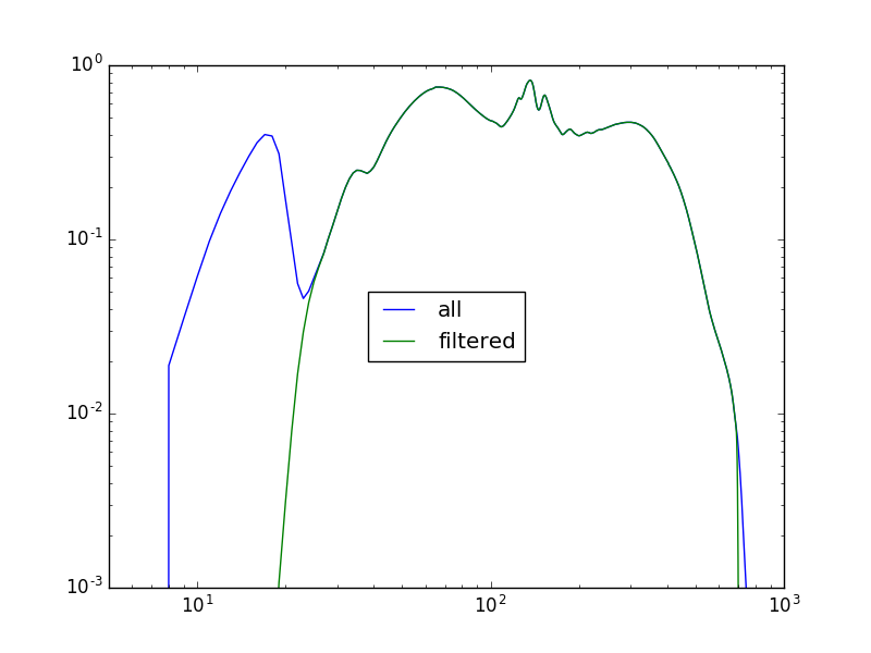
When evaluate, over whole 1-1024 channels, but can take advantage of the filter if within a setup block (this is performed automatically by certain routines, such as a fit):
>>> y1 = inst([])
>>> inst.setup()
>>> y2 = inst([])
>>> y1.size, y2.size
(1024, 1024)
>>> np.all(y1 == y2)
>>> x = np.arange(1, 1025)
>>> plt.plot(x, y1, label='all')
>>> plt.plot(x, y2, label='filtered')
>>> plt.xscale('log')
>>> plt.yscale('log')
>>> plt.ylim(0.001, 1)
>>> plt.xlim(5, 1000)
>>> plt.legend(loc='center')
Why is the exposure time not being included?
Or maybe this?
This could come first, although maybe need a separate section on how to use astro.instruments (since this is geeting quite long now).
>>> from sherpa.astro.io import read_pha
>>> from sherpa.models.basic import PowLaw1D
>>> pha = read_pha('3c273.pi')
>>> pl = PowLaw1D()
>>> from sherpa.astro.instrument import Response1D, RSPModelPHA
>>> rsp = Response1D(pha)
>>> mdl = rsp(pl)
>>> isinstance(mdl, RSPModelPHA)
>>> print(mdl)
apply_rmf(apply_arf((38564.608926889 * powlaw1d)))
   Param        Type          Value          Min          Max      Units
   -----        ----          -----          ---          ---      -----
   powlaw1d.gamma thawed            1          -10           10
   powlaw1d.ref frozen            1 -3.40282e+38  3.40282e+38
   powlaw1d.ampl thawed            1            0  3.40282e+38
Note that the exposure time - taken from the PHA or the ARF - is included so that the normalization is correct.