Last modified: February 26, 2007
This thread uses PINTofALE to generate a simulated Chandra spectrum. The Chandra ARF and RMF used were obtained from the Chandra Proposal Information page and placed in !ARDB. Here, we will generate an ACIS-I spectrum for a star that has a nominal ROSAT/PSPC count-rate of 0.1 ct/s (you must have PIMMS installed locally to do this). The steps involved are:
#	start IDL
idl

;	set up the PoA environment ;
.run initale

;NOTE:
;	if INITALE fails, run the script
;	@PoA_constructor

;	Change some of the preset defaults to values reasonable
;	for this exercize
!LDBDIR='$SPEX'
	;Warning: APED emissivities include ion balance from
	;Mazzotta et al., and abundances from Anders & Grevesse.
	;Care must be taken to not include them twice:
	if strpos(strlowcase(!LDBDIR),'aped',0) ge 0 then !IONEQF='none'
	if strpos(strlowcase(!LDBDIR),'aped',0) ge 0 then $
		!ABUND = !ABUND/getabund('anders & grevesse')
!NH=3e20
;	A Differential Emission Measure (DEM) is required to estimate
;	the amount of emission at any given temperature.  Typically
;	a 2-temperature model is used, as in the example below:
!DEM = mk_dem('delta', logT=!LOGT, pardem=alog10([7.55e6, 23.4e6]),$
	indem=[5.1d12,6.1d12]*0.05)

;	NOTE: the above is the only option available in the
;	chandra_acis_ao7.par file.

;	In general, stellar coronal plasmas are characterized by a
;	multi-temperature emission measure.  It is possible to
;	define a DEM from scratch interactively, using MK_DEM
;	(left click to define points along a DEM curve, and
;	right click to exit)
;
!DEM = mk_dem('cursor', logT=!LOGT, pardem=[1e10,1e14], $
  xcur=mk_dem_xcur, ycur=mk_dem_ycur)

;	A DEM thus derived may be edited in detail with DEMACS
;
!DEM = demacs(!LOGT, DEM0=!DEM, logT0=!LOGT, group=group, igroup=igroup)

;	more complicated DEMs, (e.g., splines) may also be defined:
;
in_pardem=[3.00000,4.01421,5.35229,5.49464,6.46261,7.06759,7.40923]
in_indem=[500.050,188.068,2.71397,2.16901,159.778,24.0164,0.133006]*1e11
!DEM = mk_dem('spline', logT=!LOGT, indem=in_indem, pardem=in_pardem) > 0

;	for the sake of definiteness, we will use a 2-temperature
;	delta-function emission measure distribution in the following
;	example.

T_components  = [6.9,    7.4]		;log(T[K]) components in the EM
EM_components = [5.1d12, 6.1d12]	;Emission Measure [cm^-3]
!DEM=mk_dem('delta',logT=!LOGT,pardem=T_components,indem=EM_components)

plot,!logT,!DEM,xtitle='log!d10!n(T [K])',ytitle='DEM [cm!u-5!n/logK]'

;NOTE:
;	this is a completely arbitrary DEM(T), and its only saving
;	grace is that it looks sensible.  It definitely would not
;	generate the correct number of ROSAT counts and must be
;	renormalized.
;	We will assume that a ROSAT/PSPC count rate is available,
;	and that the simulation will match this rate.  Data from
;	other missions such as ASCA, BeppoSAX, etc. can be dealt
;	with in the same manner.

;	First find and read in the ROSAT/PSPC effective area
;	you will need to know where your local PIMMS installation
;	is to do this.
;
pimmsdir = '/soft/pimms/data'	;<<<change to your local installation
rosat_pspc_open = get_pimms_file('ROSAT','PSPC','OPEN',pdir=pimmsdir)
;
rd_pimms_file, rosat_pspc_open, pspc_effar, pspc_wvlar, /wave

;	make sure that the wavelengths are sorted in increasing order
;
ae=sort(pspc_wvlar) & pspc_wvlar=pspc_wvlar[ae] & pspc_effar=pspc_effar[ae]

;	some initializations
;
src_DIST=10.	;place the source (say) 10 pc away

;	the DEM needed for the script MAKE_SPECTRUM (which will
;	be called below) must be the DEM defined at the source
;	(distance will be corrected for within the script).  Hence,
;	rescale the currently defined DEM (which has reasonable
;	values for a DEM "at Earth").
;
src_DCOR = 10.D^(alog10(4.*!DPI)+2.*alog10(src_DIST*3.1d18))
!DEM = !DEM * src_DCOR

;	now make a ROSAT/PSPC spectrum using MAKE_SPECTRUM,
;	which is a script and requires that its inputs be
;	in specially named variables and have the correct
;	units.  A more flexible approach is outlined in the
;	example sessions.
;
v_LOGT=!LOGT			;temperature grid
v_DEM=!DEM			;DEM in [cm^-3]
v_DIST=src_DIST			;distance in [pc]
v_EFFAR=pspc_effar > 0		;effective area in [cm^2]
v_WVLAR=pspc_wvlar		;effective area wavelength grid in [Ang]
v_WGRID=mid2bound(pspc_wvlar)	;sorted wavelength bin boundaries in [Ang]
v_EXPTIME=50.			;nominal exposure time [ks] (say)
v_RMF='none'			;name of OGIP-compatible RMF
;
;NOTE:
;	note that convolving with an RMF is unnecessary at this stage
;	because all we need is a total count rate estimate
;
.run make_spectrum

;	get the total count-rate and normalize the DEM to the
;	"observed" rate of 0.1 ct/s
;
obs_rate = 0.1					;[ct/s]
pred_rate = total(v_flxspc/v_EXPTIME/1e3)	;[ct/s]
print,'normalization factor: ',obs_rate/pred_rate
;normalization factor:     0.0030849559
!DEM = !DEM * obs_rate/pred_rate
;	first read in the Chandra ACIS-I on-axis ARF
;
acisi_effar=rdarf(!ARDB+'/acisi_aimpt_cy07.arf',arstr)

;	figure out the spectral binning required
;
elo=arstr.ELO & ehi=arstr.EHI & wlo=12.3985/ehi & whi=12.3985/elo

;	now reverse such that wavelengths are in increasing order
;
wlo=reverse(wlo) & whi=reverse(whi) & acisi_effar=reverse(acisi_effar)
wgrid=[wlo,max(whi)] & midwvl=0.5*(wgrid+wgrid[1:*])

;	set up to call MAKE_SPECTRUM again
;
v_LOGT=!LOGT			;temperature grid
v_DEM=!DEM			;DEM in [cm^-3]
v_EFFAR=acisi_effar		;effective area in [cm^2]
v_WVLAR=midwvl			;effective area wavelength grid in [Ang]
v_WGRID=wgrid			;sorted wavelength bin boundaries in [Ang]
v_EXPTIME=50.			;nominal exposure time [ks]
v_RMF=!ARDB+'/acisi_aimpt_cy07.rmf'	;name of OGIP-compatible RMF

;	and make the observed counts spectrum
;
.run make_spectrum

;	simulate an actual observation by finding Poisson deviates
;
nbin=n_elements(v_CTSPC)
sim_spec=intarr(nbin)
for i=0L,nbin-1L do $
  if v_CTSPC[i] gt 0 then sim_spec[i]=randomu(seed,poisson=v_CTSPC[i])

;	plot
;
plot,v_CHAN,v_CTSPC,xtitle='[keV]',ytitle='[ct]',/xl,xr=[0.5,7],$
  /yl,yr=[0.1,300],thick=2
oplot,v_CHAN,sim_spec,psym=10,thick=2,color=3
;	First note that the above results are consistent with rough
;	PIMMS results.  For a ROSAT/PSPC count rate of 0.1 ct/s,
;	a Raymond-Smith spectrum of temperature 0.54 keV produces
;	approx 0.14 ct/s with Chandra/ACIS-I.  This is within a
;	factor of 2 of the value predicted here:
;
print,total(v_CTSPC)/v_EXPTIME/1e3
;        0.174697957

;	MARX requires a spectrum in an ASCII file of 2 columns,
;	with column 1 containing the energy grid in [keV] and
;	column 2 containing the flux density in [ph/s/cm^2/keV]

;	Now, v_LINSPC[v_WVLS] and v_CONSPC[v_WVLS] are already
;	almost in this form.  They must be converted from
;	[ph/s/cm^2/bin] to [ph/s/cm^2/keV].  A point to note is
;	that v_WVLS was derived within MAKE_SPECTRUM as the
;	mid-bin value of the bin boundaries in v_WGRID.

;	convert from [Ang] to [keV]
;
v_ENERGY=12.3985/v_WVLS
Egrid=12.3985/v_WGRID

;	and get the bin width
;
dE=abs(Egrid[1:*]-Egrid)

;	derive MARX compatible flux density
;
spec_MARX = (v_LINSPC + v_CONSPC) / dE

;	reverse the arrays (so that they are in increasing order of energy)
;
spec_MARX = reverse(spec_MARX)
v_ENERGY  = reverse(v_ENERGY)

;	and print out to file
;
openw,umarx,'spec_marx.dat',/get_lun
for i=0L,n_elements(v_ENERGY)-1L do printf,umarx,v_ENERGY[i],spec_MARX[i]
close,umarx & free_lun,umarx

;	see the MARX manual at http://space.mit.edu/ASC/MARX/
;	for details on how to obtain and run MARX.  Note that updating
;       to MARX 4.2.0 will allow for for Cycle 7 simulations including ACIS
;	contamination (this will be necessary to match the ARF used in this
;	example).
;
;	We have run MARX independently on the spectrum written out
;	above, using the recipe prescribed in section 5 of the manual.
;
;	cp /soft/marx/marx.par .
;	pset marx.par ExposureTime=50000 OutputDir='sim_marx' \
;	  GratingType='NONE' DetectorType='ACIS-I' SourceFlux=-1 \
;	  SpectrumType='FILE' SpectrumFile='spec_marx.dat' \
;	  SourceType='POINT' DitherModel='INTERNAL'
;	marx TSTART=2006.46
;	marx2fits sim_marx/ spec_marx.evt
;	dmextract infile="spec_marx.evt[EVENTS][(x,y)=circle(4018,4141,10)]
;         [bin pi=1:1024:1]" outfile="spec_marx.pi" clobber=yes verbose=2

;	now read in the binned spectrum from the MARX simulation
M_CTSPC=mrdfits('spec_marx.pi',1,hdr)

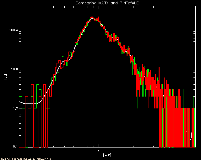
;	and overplot (in red) on the PINTofALE simulation (green)
;	(note that we do not expect perfect agreement because we have
;	used a very rough ARF in section 3 above.  nevertheless, the
;	agreement is good.)
;
plot,v_CHAN,v_CTSPC,/xl,xr=[0.2,7],/xs,/yl,yr=[0.1,400],/ys,thick=2,$
  xtitle='[keV]',ytitle='[ct]',title='Comparing MARX and PINTofALE'
oplot,v_CHAN,sim_spec,psym=10,color=3
oplot,v_CHAN,M_CTSPC.COUNTS,psym=10,thick=2,color=2
