pquad.f:1.72:
      subroutine pquad (f, a, b, absacc, relacc, minrul, maxrul,ruleno,
Error: Invalid character in name at (1)
      subroutine pquad (f, a, b, absacc, relacc, minrul, maxrul,ruleno,
&     quads, nevals, ercode)
      subroutine pquad (f, a, b, absacc, relacc, minrul,maxrul,ruleno,
     &quads, nevals, ercode)
prompt> set newpath = `echo $PATH | sed 's,/opt/local/bin:,,g'`
prompt> set path = ( /usr/bin $newpath )
prompt> make clean ; make BEHR
References
- Park, T., Kashyap, V.L., Siemiginowska, A., van Dyk, D., Zezas, A., Heinke, C., & Wargelin, B.J., 2006, ApJ, 652, 610
- preprint from 2006-jun-10:
[.ps]
[.pdf]
- [NASA Classic ADS]
- [NASA New ADS]
- [NASA Classic ADS]
- Park, T., Kashyap, V., Zezas, A., Siemiginowska, A., van Dyk, D., Connors, A., & Heinke, C., 2005, at Six Years of Science with Chandra Symposium, Nov 2-5, 2005, #5.6
- Abstract
- Poster [.ps]
- Poster [.ps]
- van Dyk, D.A., Park, T., Kashyap, V.L., \& Zezas, A., 2004, AAS-HEAD #8, 16.27
- Abstract
- Poster [.pdf]
- Poster [.pdf]
Usage and Syntax
How To
- BEHR is optimized to run as a batch job
- all the parameters are input via the command line.
- Each parameter must be explicitly specified
- e.g., softsrc=10 softbkg=100 softarea=1000, etc.
- soft and hard are terms used arbitrarily to denote passbands, and no checks are carried out to verify that they are appropriate terms.
- The two passbands must not overlap.
- *src are the counts within the source region, and *bkg are counts within the background region. These are necessarily whole numbers. The ratio of the area of the background region to the area of the source region can be passed to the program via *area.
- *eff can take into account variations in effective area and exposure times between different observations, or if all calculations must be normalized to a specific instrument.
- e.g., if the hardness ratios of ACIS-S data need to be transformed to be
comparable with hardness ratios of ACIS-I data obtained on-axis, then
softeff and hardeff can be set as unity for ACIS-I
data, and as ratios of the ACIS-S to ACIS-I instrument effective areas
for ACIS-S data in such a way as to correct for the different low-energy
response of the ACIS-S.
- The default values are generally reliable, but note some practical points:
- If working predominantly with HR, the choice for the
prior index, softidx=hardidx=1 is preferred due
to numerical stability issues.
- Use algo=quad if the net counts in either band drop below approximately 15, unless the counts in one band are very large (>100), in which case use algo=gibbs with >5x the default nsim.
- Use algo=quad if the net counts in either band drop below approximately 15, unless the counts in one band are very large (>100), in which case use algo=gibbs with >5x the default nsim.
- *idx and *scl define gamma-function priors. But starting with the 2007aug16 version, there is a provision to incorporate a user-defined table as a multiplicative function to modify the prior.
- This tabulated prior is specified via the keywords
softtbl and hardtbl and is currently implemented
only for the case algo=gibbs.
- The table must be in ASCII, and has a specific format:
line 1: NUMBER_OF_ENTRIES
line 2: the column names, usualy "lamS Pr_lamS" or something of that sort
(can be anything; this line is skipped while the file is read in).
lines 3-EOF: two columns, listing the Poisson source intensity and the
corresponding probability density
- Here is an example:
200
lamS Pr_lamS
0.0375 7.936477e-08
0.1125 5.964042e-06
0.1875 4.269368e-05
0.2625 1.521611e-04
0.3375 3.857531e-04
..........................
14.7375 7.817522e-04
14.8125 7.401423e-04
14.8875 7.006752e-04
14.9625 6.632454e-04
The first line is the number of points for the intensity. In the example, we have 200 points for the intensity. The second line is the variable names, where the first column is the intensity and the second column is the probability at the intensity. The tabulated prior distribution begins with the third line and ends with the last line (which should be line 202).- When propagating the posterior probability distribution from one calculation as the prior density for another, these tables can be used as a better means of specifying the priors than the usual gamma-function priors. In such a case, set *idx=1 and *scl=0.
- The table must be in ASCII, and has a specific format:
- A standalone IDL wrapper function called behr_hug() that calls BEHR is available via PINTofALE. Simply copy this file to your local directory to run it. It does not require any additional programs.
- An example IDL program that reads from an ASCII
input file,
calls behr_hug(),
and plots the results,
is also available (also requires IDLAstro library routines) :
behr_test.pro
- The input file, behr_test.inp, is assumed to contain whitespace separated columns of:
- soft-band counts in source region
- hard-band counts in source region
- soft-band counts in background region
- hard-band counts in background region
- ratio of background-to-source area for soft-band
- ratio of background-to-source area for hard-band
- Both behr_hug.pro and behr_test.pro and the example input file behr_test.inp are available via the tar file in subdirectory BEHR/idl/.
- Running behr_test.pro on the data in behr_test.inp, results in the following output. The various quantities calculated by BEHR such as the modes of S, H, R, C, and the mean of HR are plotted along with their error bars.
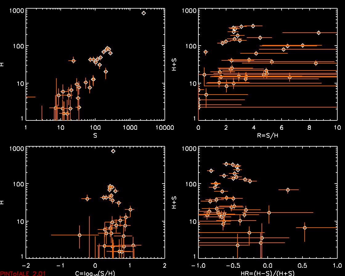
- The input file, behr_test.inp, is assumed to contain whitespace separated columns of:
- A bug that resulted in some HR upper bounds to be pegged at 0 has been corrected in the 28-aug-2012 version
-
Bug! [2012-may-17]- Mark Burke discovered that in some cases the upper bound for HR gets pegged consistently at 0 for algo=gibbs and levels>70. We have not tracked down this bug yet, but here is a workaround:
- set outputMC=true, which will produce a 2-column file of posterior draws of the source intensities in the two bands.
- compute HR=(H-S)/(H+S), sort it, and pick out the appropriate
rows to get the equal-tail error range. This can be done on the UNIX
command line, as follows:
cat output_draws.txt | awk '{print ($2-$1)/($2+$1)*1e5}' | sort -n | head -125 | tail -1 | awk '{print $1/1e5}'
cat output_draws.txt | awk '{print ($2-$1)/($2+$1)*1e5}' | sort -n | head -4875 | tail -1 | awk '{print $1/1e5}'
which returns the equal-tail 95% interval as the 2.5th and 97.5th percentiles assuming 5000 draws. The multiplication and subsequent division by 1e5 are just so sort is not confused by exponential notations.
- Mark Burke discovered that in some cases the upper bound for HR gets pegged consistently at 0 for algo=gibbs and levels>70. We have not tracked down this bug yet, but here is a workaround:
| Code | References | Usage | How to |
[CHASC]